data representation techniques in computer

• School Guide
• Mathematics
• Number System and Arithmetic
• Trigonometry
• Probability
• Mensuration
• Maths Formulas
• Class 8 Maths Notes
• Class 9 Maths Notes
• Class 10 Maths Notes
• Class 11 Maths Notes
• Class 12 Maths Notes
• What are the rational numbers between 3 and 5?
• In how many ways a committee of 3 can be made from a total of 10 members?
• Which kind of angle is between the smallest and the largest?
• How many bit strings of length 9 have exactly 4 0's?
• What are non negative real numbers?
• Is 0.5 a whole number?
• What is 2i equal to?
• What are the six trigonometry functions?
• What is the magnitude of the complex number 3 - 2i?
• What are the uses of arithmetic mean?
• How to find the ratio in which a point divides a line?
• Evaluate sin 35° sin 55° - cos 35° cos 55°
• If tan (A + B) = √3 and tan (A – B) = 1/√3, 0° B, then find A and B
• How to find the vertex angle?
• What is the most likely score from throwing two dice?
• If two numbers a and b are even, then prove that their sum a + b is even
• State whether Every whole number is a natural number or not
• How to convert a complex number to exponential form?
• What happens when you subtract two negatives?

What are the different ways of Data Representation?

The process of collecting the data and analyzing that data in large quantity is known as statistics. It is a branch of mathematics trading with the collection, analysis, interpretation, and presentation of numeral facts and figures.

It is a numerical statement that helps us to collect and analyze the data in large quantity the statistics are based on two of its concepts:

• Statistical Data 
• Statistical Science

Statistics must be expressed numerically and should be collected systematically.

Data Representation

The word data refers to constituting people, things, events, ideas. It can be a title, an integer, or anycast.  After collecting data the investigator has to condense them in tabular form to study their salient features. Such an arrangement is known as the presentation of data.

It refers to the process of condensing the collected data in a tabular form or graphically. This arrangement of data is known as Data Representation.

The row can be placed in different orders like it can be presented in ascending orders, descending order, or can be presented in alphabetical order. 

Example: Let the marks obtained by 10 students of class V in a class test, out of 50 according to their roll numbers, be: 39, 44, 49, 40, 22, 10, 45, 38, 15, 50 The data in the given form is known as raw data. The above given data can be placed in the serial order as shown below: Roll No. Marks 1 39 2 44 3 49 4 40 5 22 6 10 7 45 8 38 9 14 10 50 Now, if you want to analyse the standard of achievement of the students. If you arrange them in ascending or descending order, it will give you a better picture. Ascending order: 10, 15, 22, 38, 39, 40, 44. 45, 49, 50 Descending order: 50, 49, 45, 44, 40, 39, 38, 22, 15, 10 When the row is placed in ascending or descending order is known as arrayed data.

Types of Graphical Data Representation

Bar chart helps us to represent the collected data visually. The collected data can be visualized horizontally or vertically in a bar chart like amounts and frequency. It can be grouped or single. It helps us in comparing different items. By looking at all the bars, it is easy to say which types in a group of data influence the other.

Now let us understand bar chart by taking this example  Let the marks obtained by 5 students of class V in a class test, out of 10 according to their names, be: 7,8,4,9,6 The data in the given form is known as raw data. The above given data can be placed in the bar chart as shown below: Name Marks Akshay 7 Maya 8 Dhanvi 4 Jaslen 9 Muskan 6

A histogram is the graphical representation of data. It is similar to the appearance of a bar graph but there is a lot of difference between histogram and bar graph because a bar graph helps to measure the frequency of categorical data. A categorical data means it is based on two or more categories like gender, months, etc. Whereas histogram is used for quantitative data.

For example:

The graph which uses lines and points to present the change in time is known as a line graph. Line graphs can be based on the number of animals left on earth, the increasing population of the world day by day, or the increasing or decreasing the number of bitcoins day by day, etc. The line graphs tell us about the changes occurring across the world over time. In a  line graph, we can tell about two or more types of changes occurring around the world.

For Example:

Pie chart is a type of graph that involves a structural graphic representation of numerical proportion. It can be replaced in most cases by other plots like a bar chart, box plot, dot plot, etc. As per the research, it is shown that it is difficult to compare the different sections of a given pie chart, or if it is to compare data across different pie charts.

Frequency Distribution Table

A frequency distribution table is a chart that helps us to summarise the value and the frequency of the chart. This frequency distribution table has two columns, The first column consist of the list of the various outcome in the data, While the second column list the frequency of each outcome of the data. By putting this kind of data into a table it helps us to make it easier to understand and analyze the data. 

For Example: To create a frequency distribution table, we would first need to list all the outcomes in the data. In this example, the results are 0 runs, 1 run, 2 runs, and 3 runs. We would list these numerals in numerical ranking in the foremost queue. Subsequently, we ought to calculate how many times per result happened. They scored 0 runs in the 1st, 4th, 7th, and 8th innings, 1 run in the 2nd, 5th, and the 9th innings, 2 runs in the 6th inning, and 3 runs in the 3rd inning. We set the frequency of each result in the double queue. You can notice that the table is a vastly more useful method to show this data.  Baseball Team Runs Per Inning Number of Runs Frequency           0       4           1        3            2        1            3        1

Sample Questions

Question 1: Considering the school fee submission of 10 students of class 10th is given below:

In order to draw the bar graph for the data above, we prepare the frequency table as given below. Fee submission No. of Students Paid   6 Not paid    4 Now we have to represent the data by using the bar graph. It can be drawn by following the steps given below: Step 1: firstly we have to draw the two axis of the graph X-axis and the Y-axis. The varieties of the data must be put on the X-axis (the horizontal line) and the frequencies of the data must be put on the Y-axis (the vertical line) of the graph. Step 2: After drawing both the axis now we have to give the numeric scale to the Y-axis (the vertical line) of the graph It should be started from zero and ends up with the highest value of the data. Step 3: After the decision of the range at the Y-axis now we have to give it a suitable difference of the numeric scale. Like it can be 0,1,2,3…….or 0,10,20,30 either we can give it a numeric scale like 0,20,40,60… Step 4: Now on the X-axis we have to label it appropriately. Step 5: Now we have to draw the bars according to the data but we have to keep in mind that all the bars should be of the same length and there should be the same distance between each graph

Question 2: Watch the subsequent pie chart that denotes the money spent by Megha at the funfair. The suggested colour indicates the quantity paid for each variety. The total value of the data is 15 and the amount paid on each variety is diagnosed as follows:

Chocolates – 3

Wafers – 3

Toys – 2

Rides – 7

To convert this into pie chart percentage, we apply the formula:  (Frequency/Total Frequency) × 100 Let us convert the above data into a percentage: Amount paid on rides: (7/15) × 100 = 47% Amount paid on toys: (2/15) × 100 = 13% Amount paid on wafers: (3/15) × 100 = 20% Amount paid on chocolates: (3/15) × 100 = 20 %

Question 3: The line graph given below shows how Devdas’s height changes as he grows.

Given below is a line graph showing the height changes in Devdas’s as he grows. Observe the graph and answer the questions below.

(i) What was the height of  Devdas’s at 8 years? Answer: 65 inches (ii) What was the height of  Devdas’s at 6 years? Answer:  50 inches (iii) What was the height of  Devdas’s at 2 years? Answer: 35 inches (iv) How much has  Devdas’s grown from 2 to 8 years? Answer: 30 inches (v) When was  Devdas’s 35 inches tall? Answer: 2 years.

Please Login to comment...

• School Learning
• School Mathematics
• What Is Trunk-Or-Treat?
• 10 Best AI Tools for Lawyers (Free + Paid)
• Fireflies AI vs Gong: Which AI Tool is best in 2024?
• Top 10 Alternatives to Snapseed in 2024 [Free + Paid]
• 30 OOPs Interview Questions and Answers (2024)

Improve your Coding Skills with Practice

What kind of Experience do you want to share?

Data representation 1: Introduction

This course investigates how systems software works: what makes programs work fast or slow, and how properties of the machines we program impact the programs we write. We discuss both general ideas and specific tools, and take an experimental approach.

Textbook readings

• How do computers represent different kinds of information?
• How do data representation choices impact performance and correctness?
• What kind of language is understood by computer processors?
• How is code you write translated to code a processor runs?
• How do hardware and software defend against bugs and attacks?
• How are operating systems interfaces implemented?
• What kinds of computer data storage are available, and how do they perform?
• How can we improve the performance of a system that stores data?
• How can programs on the same computer cooperate and interact?
• What kinds of operating systems interfaces are useful?
• How can a single program safely use multiple processors?
• How can multiple computers safely interact over a network?
• Six problem sets
• Midterm and final
• Starting mid-next week
• Attendance checked for simultaneously-enrolled students
• Rough breakdown: >50% assignments, <35% tests, 15% participation
• Course grading: A means mastery

Collaboration

Discussion, collaboration, and the exchange of ideas are essential to doing academic work, and to engineering. You are encouraged to consult with your classmates as you work on problem sets. You are welcome to discuss general strategies for solutions as well as specific bugs and code structure questions, and to use Internet resources for general information.

However, the work you turn in must be your own—the result of your own efforts. You should understand your code well enough that you could replicate your solution from scratch, without collaboration.

In addition, you must cite any books, articles, online resources, and so forth that helped you with your work, using appropriate citation practices; and you must list the names of students with whom you have collaborated on problem sets and briefly describe how you collaborated. (You do not need to list course staff.)

On our programming language

We use the C++ programming language in this class.

C++ is a boring, old, and unsafe programming language, but boring languages are underrated . C++ offers several important advantages for this class, including ubiquitous availability, good tooling, the ability to demonstrate impactful kinds of errors that you should understand, and a good standard library of data structures.

Pset 0 links to several C++ tutorials and references, and to a textbook.

Each program runs in a private data storage space. This is called its memory . The memory “remembers” the data it stores.

Programs work by manipulating values . Different programming languages have different conceptions of value; in C++, the primitive values are integers, like 12 or -100; floating-point numbers, like 1.02; and pointers , which are references to other objects.

An object is a region of memory that contains a value. (The C++ standard specifically says “a region of data storage in the execution environment, the contents of which can represent values”.)

Objects, values, and variables

Which are the objects? Which are the values?

Variables generally correspond to objects, and here there are three objects, one for each variable i1 , i2 , and i3 . The compiler and operating system associate the names with their corresponding objects. There are three values, too, one used to initialize each object: 61 , 62 , and 63 . However, there are other values—for instance, each argument to the printf calls is a value.

What does the program print?

i1: 61 i2: 62 i3: 63

C and C++ pointer types allow programs to access objects indirectly. A pointer value is the address of another object. For instance, in this program, the variable i4 holds a pointer to the object named by i3 :

There are four objects, corresponding to variables i1 through i4 . Note that the i4 object holds a pointer value, not an integer. There are also four values: 61 , 62 , 63 , and the expression &i3 (the address of i3 ). Note that there are three integer values, but four values overall.

What does this program print?

i1: 61 i2: 62 i3: 63 value pointed to by i4: 63

Here, the expressions i3 and *i4 refer to exactly the same object. Any modification to i3 can be observed through *i4 and vice versa. We say that i3 and *i4 are aliases : different names for the same object.

We now use hexdump_object , a helper function declared in our hexdump.hh helper file , to examine both the contents and the addresses of these objects.

Exactly what is printed will vary between operating systems and compilers. In Docker in class, on my Apple-silicon Macbook, we saw:

But on an Intel-based Amazon EC2 native Linux machine:

The data bytes look similar—identical for i1 through i3 —but the addresses vary.

But on Intel Mac OS X: 103c63020 3d 00 00 00 |=...| 103c5ef60 3e 00 00 00 |>...| 7ffeebfa4abc 3f 00 00 00 |?...| 7ffeebfa4ab0 bc 4a fa eb fe 7f 00 00 |.J......| And on Docker on an Intel Mac: 56499f239010 3d 00 00 00 |=...| 56499f23701c 3e 00 00 00 |>...| 7fffebf8b19c 3f 00 00 00 |?...| 7fffebf8b1a0 9c b1 f8 eb ff 7f 00 00 |........|

A hexdump printout shows the following information on each line.

• An address , like 4000004010 . This is a hexadecimal (base-16) number indicating the value of the address of the object. A line contains one to sixteen bytes of memory starting at this address.
• The contents of memory starting at the given address, such as 3d 00 00 00 . Memory is printed as a sequence of bytes , which are 8-bit numbers between 0 and 255. All modern computers organize their memory in units of 8-bit bytes.
• A textual representation of the memory contents, such as |=...| . This is useful when examining memory that contains textual data, and random garbage otherwise.

Dynamic allocation

Must every data object be given a name? No! In C++, the new operator allocates a brand-new object with no variable name. (In C, the malloc function does the same thing.) The C++ expression new T returns a pointer to a brand-new, never-before-seen object of type T . For instance:

This prints something like

The new int{64} expression allocates a fresh object with no name of its own, though it can be located by following the i4 pointer.

What do you notice about the addresses of these different objects?

• i3 and i4 , which are objects corresponding to variables declared local to main , are located very close to one another. In fact they are just 4 bytes part: i3 directly abuts i4 . Their addresses are quite high. In native Linux, in fact, their addresses are close to 2 47 !
• i1 and i2 are at much lower addresses, and they do not abut. i2 ’s location is below i1 , and about 0x2000 bytes away.
• The anonymous storage allocated by new int is located between i1 / i2 and i3 / i4 .

Although the values may differ on other operating systems, you’ll see qualitatively similar results wherever you run ./objects .

What’s happening is that the operating system and compiler have located different kinds of object in different broad regions of memory. These regions are called segments , and they are important because objects’ different storage characteristics benefit from different treatment.

i2 , the const int global object, has the smallest address. It is in the code or text segment, which is also used for read-only global data. The operating system and hardware ensure that data in this segment is not changed during the lifetime of the program. Any attempt to modify data in the code segment will cause a crash.

i1 , the int global object, has the next highest address. It is in the data segment, which holds modifiable global data. This segment keeps the same size as the program runs.

After a jump, the anonymous new int object pointed to by i4 has the next highest address. This is the heap segment, which holds dynamically allocated data. This segment can grow as the program runs; it typically grows towards higher addresses.

After a larger jump, the i3 and i4 objects have the highest addresses. They are in the stack segment, which holds local variables. This segment can also grow as the program runs, especially as functions call other functions; in most processors it grows down , from higher addresses to lower addresses.

Experimenting with the stack

How can we tell that the stack grows down? Do all functions share a single stack? This program uses a recursive function to test. Try running it; what do you see?

• FOUNDATION YEARS
• LEARN TO CODE
• ROBOTICS ENGINEERING
• CLASS PROJECTS
• Classroom Discussions
• Useful Links

Data representation

Computers use binary - the digits 0 and 1 - to store data. A binary digit, or bit, is the smallest unit of data in computing. It is represented by a 0 or a 1. Binary numbers are made up of binary digits (bits), eg the binary number 1001. The circuits in a computer's processor are made up of billions of transistors. A transistor is a tiny switch that is activated by the electronic signals it receives. The digits 1 and 0 used in binary reflect the on and off states of a transistor. Computer programs are sets of instructions. Each instruction is translated into machine code - simple binary codes that activate the CPU. Programmers write computer code and this is converted by a translator into binary instructions that the processor can execute. All software, music, documents, and any other information that is processed by a computer, is also stored using binary. [1]

To include strings, integers, characters and colours. This should include considering the space taken by data, for instance the relation between the hexadecimal representation of colours and the number of colours available.

This video is superb place to understand this topic

• 1 How a file is stored on a computer
• 2 How an image is stored in a computer
• 3 The way in which data is represented in the computer.
• 6 Standards
• 7 References

How a file is stored on a computer [ edit ]

How an image is stored in a computer [ edit ]

The way in which data is represented in the computer. [ edit ].

To include strings, integers, characters and colours. This should include considering the space taken by data, for instance the relation between the hexadecimal representation of colours and the number of colours available [3] .

This helpful material is used with gratitude from a computer science wiki under a Creative Commons Attribution 3.0 License [4]

Sound [ edit ]

• Let's look at an oscilloscope
• The BBC has an excellent article on how computers represent sound

See Also [ edit ]

Standards [ edit ].

• Outline the way in which data is represented in the computer.

References [ edit ]

• ↑ http://www.bbc.co.uk/education/guides/zwsbwmn/revision/1
• ↑ https://ujjwalkarn.me/2016/08/11/intuitive-explanation-convnets/
• ↑ IBO Computer Science Guide, First exams 2014
• ↑ https://compsci2014.wikispaces.com/2.1.10+Outline+the+way+in+which+data+is+represented+in+the+computer

A unit of abstract mathematical system subject to the laws of arithmetic.

A natural number, a negative of a natural number, or zero.

Give a brief account.

• Computer organization
• Very important ideas in computer science

Data Representation in Computer: Number Systems, Characters, Audio, Image and Video

• Post author: Anuj Kumar
• Post published: 16 July 2021
• Post category: Computer Science
• Post comments: 0 Comments

Table of Contents

• 1 What is Data Representation in Computer?
• 2.1 Binary Number System
• 2.2 Octal Number System
• 2.3 Decimal Number System
• 2.4 Hexadecimal Number System
• 3.4 Unicode
• 4 Data Representation of Audio, Image and Video
• 5.1 What is number system with example?

What is Data Representation in Computer?

A computer uses a fixed number of bits to represent a piece of data which could be a number, a character, image, sound, video, etc. Data representation is the method used internally to represent data in a computer. Let us see how various types of data can be represented in computer memory.

Before discussing data representation of numbers, let us see what a number system is.

Number Systems

Number systems are the technique to represent numbers in the computer system architecture, every value that you are saving or getting into/from computer memory has a defined number system.

A number is a mathematical object used to count, label, and measure. A number system is a systematic way to represent numbers. The number system we use in our day-to-day life is the decimal number system that uses 10 symbols or digits.

The number 289 is pronounced as two hundred and eighty-nine and it consists of the symbols 2, 8, and 9. Similarly, there are other number systems. Each has its own symbols and method for constructing a number.

A number system has a unique base, which depends upon the number of symbols. The number of symbols used in a number system is called the base or radix of a number system.

Let us discuss some of the number systems. Computer architecture supports the following number of systems:

Binary Number System

Octal number system, decimal number system, hexadecimal number system.

A Binary number system has only two digits that are 0 and 1. Every number (value) represents 0 and 1 in this number system. The base of the binary number system is 2 because it has only two digits.

The octal number system has only eight (8) digits from 0 to 7. Every number (value) represents with 0,1,2,3,4,5,6 and 7 in this number system. The base of the octal number system is 8, because it has only 8 digits.

The decimal number system has only ten (10) digits from 0 to 9. Every number (value) represents with 0,1,2,3,4,5,6, 7,8 and 9 in this number system. The base of decimal number system is 10, because it has only 10 digits.

A Hexadecimal number system has sixteen (16) alphanumeric values from 0 to 9 and A to F. Every number (value) represents with 0,1,2,3,4,5,6, 7,8,9,A,B,C,D,E and F in this number system. The base of the hexadecimal number system is 16, because it has 16 alphanumeric values.

Here A is 10, B is 11, C is 12, D is 13, E is 14 and F is 15 .

Data Representation of Characters

There are different methods to represent characters . Some of them are discussed below:

The code called ASCII (pronounced ‘􀀏’.S-key”), which stands for American Standard Code for Information Interchange, uses 7 bits to represent each character in computer memory. The ASCII representation has been adopted as a standard by the U.S. government and is widely accepted.

A unique integer number is assigned to each character. This number called ASCII code of that character is converted into binary for storing in memory. For example, the ASCII code of A is 65, its binary equivalent in 7-bit is 1000001.

Since there are exactly 128 unique combinations of 7 bits, this 7-bit code can represent only128 characters. Another version is ASCII-8, also called extended ASCII, which uses 8 bits for each character, can represent 256 different characters.

For example, the letter A is represented by 01000001, B by 01000010 and so on. ASCII code is enough to represent all of the standard keyboard characters.

It stands for Extended Binary Coded Decimal Interchange Code. This is similar to ASCII and is an 8-bit code used in computers manufactured by International Business Machines (IBM). It is capable of encoding 256 characters.

If ASCII-coded data is to be used in a computer that uses EBCDIC representation, it is necessary to transform ASCII code to EBCDIC code. Similarly, if EBCDIC coded data is to be used in an ASCII computer, EBCDIC code has to be transformed to ASCII.

ISCII stands for Indian Standard Code for Information Interchange or Indian Script Code for Information Interchange. It is an encoding scheme for representing various writing systems of India. ISCII uses 8-bits for data representation.

It was evolved by a standardization committee under the Department of Electronics during 1986-88 and adopted by the Bureau of Indian Standards (BIS). Nowadays ISCII has been replaced by Unicode.

Using 8-bit ASCII we can represent only 256 characters. This cannot represent all characters of written languages of the world and other symbols. Unicode is developed to resolve this problem. It aims to provide a standard character encoding scheme, which is universal and efficient.

It provides a unique number for every character, no matter what the language and platform be. Unicode originally used 16 bits which can represent up to 65,536 characters. It is maintained by a non-profit organization called the Unicode Consortium.

The Consortium first published version 1.0.0 in 1991 and continues to develop standards based on that original work. Nowadays Unicode uses more than 16 bits and hence it can represent more characters. Unicode can represent characters in almost all written languages of the world.

Data Representation of Audio, Image and Video

In most cases, we may have to represent and process data other than numbers and characters. This may include audio data, images, and videos. We can see that like numbers and characters, the audio, image, and video data also carry information.

We will see different file formats for storing sound, image, and video .

Multimedia data such as audio, image, and video are stored in different types of files. The variety of file formats is due to the fact that there are quite a few approaches to compressing the data and a number of different ways of packaging the data.

For example, an image is most popularly stored in Joint Picture Experts Group (JPEG ) file format. An image file consists of two parts – header information and image data. Information such as the name of the file, size, modified data, file format, etc. is stored in the header part.

The intensity value of all pixels is stored in the data part of the file. The data can be stored uncompressed or compressed to reduce the file size. Normally, the image data is stored in compressed form. Let us understand what compression is.

Take a simple example of a pure black image of size 400X400 pixels. We can repeat the information black, black, …, black in all 16,0000 (400X400) pixels. This is the uncompressed form, while in the compressed form black is stored only once and information to repeat it 1,60,000 times is also stored.

Numerous such techniques are used to achieve compression. Depending on the application, images are stored in various file formats such as bitmap file format (BMP), Tagged Image File Format (TIFF), Graphics Interchange Format (GIF), Portable (Public) Network Graphic (PNG).

What we said about the header file information and compression is also applicable for audio and video files. Digital audio data can be stored in different file formats like WAV, MP3, MIDI, AIFF, etc. An audio file describes a format, sometimes referred to as the ‘container format’, for storing digital audio data.

For example, WAV file format typically contains uncompressed sound and MP3 files typically contain compressed audio data. The synthesized music data is stored in MIDI(Musical Instrument Digital Interface) files.

Similarly, video is also stored in different files such as AVI (Audio Video Interleave) – a file format designed to store both audio and video data in a standard package that allows synchronous audio with video playback, MP3, JPEG-2, WMV, etc.

FAQs About Data Representation in Computer

What is number system with example.

Let us discuss some of the number systems. Computer architecture supports the following number of systems: 1. Binary Number System 2. Octal Number System 3. Decimal Number System 4. Hexadecimal Number System

Related posts:

• 10 Types of Computers | History of Computers, Advantages

What is Microprocessor? Evolution of Microprocessor, Types, Features

• What is operating system? Functions, Types, Types of User Interface

What is Cloud Computing? Classification, Characteristics, Principles, Types of Cloud Providers

What is debugging types of errors, what are functions of operating system 6 functions, what is flowchart in programming symbols, advantages, preparation, advantages and disadvantages of flowcharts, what is c++ programming language c++ character set, c++ tokens.

• What are C++ Keywords? Set of 59 keywords in C ++

What are Data Types in C++? Types

What are operators in c different types of operators in c, what are expressions in c types, what are decision making statements in c types, types of storage devices, advantages, examples, you might also like.

Types of Computer Software: Systems Software, Application Software

What is Problem Solving Algorithm?, Steps, Representation

10 Evolution of Computing Machine, History

What is Artificial Intelligence? Functions, 6 Benefits, Applications of AI

Data and Information: Definition, Characteristics, Types, Channels, Approaches

What is Big Data? Characteristics, Tools, Types, Internet of Things (IOT)

What is Computer System? Definition, Characteristics, Functional Units, Components

Advantages and Disadvantages of Operating System

• Entrepreneurship
• Organizational Behavior
• Financial Management
• Communication
• Human Resource Management
• Sales Management
• Marketing Management

Page Statistics

Table of contents.

• Introduction to Functional Computer
• Fundamentals of Architectural Design

Data Representation

• Instruction Set Architecture : Instructions and Formats
• Instruction Set Architecture : Design Models
• Instruction Set Architecture : Addressing Modes
• Performance Measurements and Issues
• Computer Architecture Assessment 1
• Fixed Point Arithmetic : Addition and Subtraction
• Fixed Point Arithmetic : Multiplication
• Fixed Point Arithmetic : Division
• Floating Point Arithmetic
• Arithmetic Logic Unit Design
• CPU's Data Path
• CPU's Control Unit
• Control Unit Design
• Concepts of Pipelining
• Computer Architecture Assessment 2
• Pipeline Hazards
• Memory Characteristics and Organization
• Cache Memory
• Virtual Memory
• I/O Communication and I/O Controller
• Input/Output Data Transfer
• Direct Memory Access controller and I/O Processor
• CPU Interrupts and Interrupt Handling
• Computer Architecture Assessment 3

Course Computer Architecture

Digital computers store and process information in binary form as digital logic has only two values "1" and "0" or in other words "True or False" or also said as "ON or OFF". This system is called radix 2. We human generally deal with radix 10 i.e. decimal. As a matter of convenience there are many other representations like Octal (Radix 8), Hexadecimal (Radix 16), Binary coded decimal (BCD), Decimal etc.

Every computer's CPU has a width measured in terms of bits such as 8 bit CPU, 16 bit CPU, 32 bit CPU etc. Similarly, each memory location can store a fixed number of bits and is called memory width. Given the size of the CPU and Memory, it is for the programmer to handle his data representation. Most of the readers may be knowing that 4 bits form a Nibble, 8 bits form a byte. The word length is defined by the Instruction Set Architecture of the CPU. The word length may be equal to the width of the CPU.

The memory simply stores information as a binary pattern of 1's and 0's. It is to be interpreted as what the content of a memory location means. If the CPU is in the Fetch cycle, it interprets the fetched memory content to be instruction and decodes based on Instruction format. In the Execute cycle, the information from memory is considered as data. As a common man using a computer, we think computers handle English or other alphabets, special characters or numbers. A programmer considers memory content to be data types of the programming language he uses. Now recall figure 1.2 and 1.3 of chapter 1 to reinforce your thought that conversion happens from computer user interface to internal representation and storage.

• Data Representation in Computers

Information handled by a computer is classified as instruction and data. A broad overview of the internal representation of the information is illustrated in figure 3.1. No matter whether it is data in a numeric or non-numeric form or integer, everything is internally represented in Binary. It is up to the programmer to handle the interpretation of the binary pattern and this interpretation is called Data Representation . These data representation schemes are all standardized by international organizations.

Choice of Data representation to be used in a computer is decided by

• The number types to be represented (integer, real, signed, unsigned, etc.)
• Range of values likely to be represented (maximum and minimum to be represented)
• The Precision of the numbers i.e. maximum accuracy of representation (floating point single precision, double precision etc)
• If non-numeric i.e. character, character representation standard to be chosen. ASCII, EBCDIC, UTF are examples of character representation standards.
• The hardware support in terms of word width, instruction.

Before we go into the details, let us take an example of interpretation. Say a byte in Memory has value "0011 0001". Although there exists a possibility of so many interpretations as in figure 3.2, the program has only one interpretation as decided by the programmer and declared in the program.

• Fixed point Number Representation

Fixed point numbers are also known as whole numbers or Integers. The number of bits used in representing the integer also implies the maximum number that can be represented in the system hardware. However for the efficiency of storage and operations, one may choose to represent the integer with one Byte, two Bytes, Four bytes or more. This space allocation is translated from the definition used by the programmer while defining a variable as integer short or long and the Instruction Set Architecture.

In addition to the bit length definition for integers, we also have a choice to represent them as below:

• Unsigned Integer : A positive number including zero can be represented in this format. All the allotted bits are utilised in defining the number. So if one is using 8 bits to represent the unsigned integer, the range of values that can be represented is 28 i.e. "0" to "255". If 16 bits are used for representing then the range is 216 i.e. "0 to 65535".
• Signed Integer : In this format negative numbers, zero, and positive numbers can be represented. A sign bit indicates the magnitude direction as positive or negative. There are three possible representations for signed integer and these are Sign Magnitude format, 1's Compliment format and 2's Complement format .

Signed Integer – Sign Magnitude format: Most Significant Bit (MSB) is reserved for indicating the direction of the magnitude (value). A "0" on MSB means a positive number and a "1" on MSB means a negative number. If n bits are used for representation, n-1 bits indicate the absolute value of the number. Examples for n=8:

Examples for n=8:

0010 1111 = + 47 Decimal (Positive number)

1010 1111 = - 47 Decimal (Negative Number)

0111 1110 = +126 (Positive number)

1111 1110 = -126 (Negative Number)

0000 0000 = + 0 (Postive Number)

1000 0000 = - 0 (Negative Number)

Although this method is easy to understand, Sign Magnitude representation has several shortcomings like

• Zero can be represented in two ways causing redundancy and confusion.
• The total range for magnitude representation is limited to 2n-1, although n bits were accounted.
• The separate sign bit makes the addition and subtraction more complicated. Also, comparing two numbers is not straightforward.

Signed Integer – 1’s Complement format: In this format too, MSB is reserved as the sign bit. But the difference is in representing the Magnitude part of the value for negative numbers (magnitude) is inversed and hence called 1’s Complement form. The positive numbers are represented as it is in binary. Let us see some examples to better our understanding.

1101 0000 = - 47 Decimal (Negative Number)

1000 0001 = -126 (Negative Number)

1111 1111 = - 0 (Negative Number)

• Converting a given binary number to its 2's complement form

Step 1 . -x = x' + 1 where x' is the one's complement of x.

Step 2 Extend the data width of the number, fill up with sign extension i.e. MSB bit is used to fill the bits.

Example: -47 decimal over 8bit representation

As you can see zero is not getting represented with redundancy. There is only one way of representing zero. The other problem of the complexity of the arithmetic operation is also eliminated in 2’s complement representation. Subtraction is done as Addition.

More exercises on number conversion are left to the self-interest of readers.

• Floating Point Number system

The maximum number at best represented as a whole number is 2 n . In the Scientific world, we do come across numbers like Mass of an Electron is 9.10939 x 10-31 Kg. Velocity of light is 2.99792458 x 108 m/s. Imagine to write the number in a piece of paper without exponent and converting into binary for computer representation. Sure you are tired!!. It makes no sense to write a number in non- readable form or non- processible form. Hence we write such large or small numbers using exponent and mantissa. This is said to be Floating Point representation or real number representation. he real number system could have infinite values between 0 and 1.

Representation in computer

Unlike the two's complement representation for integer numbers, Floating Point number uses Sign and Magnitude representation for both mantissa and exponent . In the number 9.10939 x 1031, in decimal form, +31 is Exponent, 9.10939 is known as Fraction . Mantissa, Significand and fraction are synonymously used terms. In the computer, the representation is binary and the binary point is not fixed. For example, a number, say, 23.345 can be written as 2.3345 x 101 or 0.23345 x 102 or 2334.5 x 10-2. The representation 2.3345 x 101 is said to be in normalised form.

Floating-point numbers usually use multiple words in memory as we need to allot a sign bit, few bits for exponent and many bits for mantissa. There are standards for such allocation which we will see sooner.

• IEEE 754 Floating Point Representation

We have two standards known as Single Precision and Double Precision from IEEE. These standards enable portability among different computers. Figure 3.3 picturizes Single precision while figure 3.4 picturizes double precision. Single Precision uses 32bit format while double precision is 64 bits word length. As the name suggests double precision can represent fractions with larger accuracy. In both the cases, MSB is sign bit for the mantissa part, followed by Exponent and Mantissa. The exponent part has its sign bit.

It is to be noted that in Single Precision, we can represent an exponent in the range -127 to +127. It is possible as a result of arithmetic operations the resulting exponent may not fit in. This situation is called overflow in the case of positive exponent and underflow in the case of negative exponent. The Double Precision format has 11 bits for exponent meaning a number as large as -1023 to 1023 can be represented. The programmer has to make a choice between Single Precision and Double Precision declaration using his knowledge about the data being handled.

The Floating Point operations on the regular CPU is very very slow. Generally, a special purpose CPU known as Co-processor is used. This Co-processor works in tandem with the main CPU. The programmer should be using the float declaration only if his data is in real number form. Float declaration is not to be used generously.

• Decimal Numbers Representation

Decimal numbers (radix 10) are represented and processed in the system with the support of additional hardware. We deal with numbers in decimal format in everyday life. Some machines implement decimal arithmetic too, like floating-point arithmetic hardware. In such a case, the CPU uses decimal numbers in BCD (binary coded decimal) form and does BCD arithmetic operation. BCD operates on radix 10. This hardware operates without conversion to pure binary. It uses a nibble to represent a number in packed BCD form. BCD operations require not only special hardware but also decimal instruction set.

• Exceptions and Error Detection

All of us know that when we do arithmetic operations, we get answers which have more digits than the operands (Ex: 8 x 2= 16). This happens in computer arithmetic operations too. When the result size exceeds the allotted size of the variable or the register, it becomes an error and exception. The exception conditions associated with numbers and number operations are Overflow, Underflow, Truncation, Rounding and Multiple Precision . These are detected by the associated hardware in arithmetic Unit. These exceptions apply to both Fixed Point and Floating Point operations. Each of these exceptional conditions has a flag bit assigned in the Processor Status Word (PSW). We may discuss more in detail in the later chapters.

• Character Representation

Another data type is non-numeric and is largely character sets. We use a human-understandable character set to communicate with computer i.e. for both input and output. Standard character sets like EBCDIC and ASCII are chosen to represent alphabets, numbers and special characters. Nowadays Unicode standard is also in use for non-English language like Chinese, Hindi, Spanish, etc. These codes are accessible and available on the internet. Interested readers may access and learn more.

1. Track your progress [Earn 200 points]

Mark as complete

2. Provide your ratings to this chapter [Earn 100 points]

Computer Science: Reflections on the Field, Reflections from the Field (2004)

Chapter: 5 data, representation, and information, 5 data, representation, and information.

T he preceding two chapters address the creation of models that capture phenomena of interest and the abstractions both for data and for computation that reduce these models to forms that can be executed by computer. We turn now to the ways computer scientists deal with information, especially in its static form as data that can be manipulated by programs.

Gray begins by narrating a long line of research on databases—storehouses of related, structured, and durable data. We see here that the objects of research are not data per se but rather designs of “schemas” that allow deliberate inquiry and manipulation. Gray couples this review with introspection about the ways in which database researchers approach these problems.

Databases support storage and retrieval of information by defining—in advance—a complex structure for the data that supports the intended operations. In contrast, Lesk reviews research on retrieving information from documents that are formatted to meet the needs of applications rather than predefined schematized formats.

Interpretation of information is at the heart of what historians do, and Ayers explains how information technology is transforming their paradigms. He proposes that history is essentially model building—constructing explanations based on available information—and suggests that the methods of computer science are influencing this core aspect of historical analysis.

DATABASE SYSTEMS: A TEXTBOOK CASE OF RESEARCH PAYING OFF

Jim Gray, Microsoft Research

A small research investment helped produce U.S. market dominance in the $14 billion database industry. Government and industry funding of a few research projects created the ideas for several generations of products and trained the people who built those products. Continuing research is now creating the ideas and training the people for the next generation of products.

Industry Profile

The database industry generated about $14 billion in revenue in 2002 and is growing at 20 percent per year, even though the overall technology sector is almost static. Among software sectors, the database industry is second only to operating system software. Database industry leaders are all U.S.-based corporations: IBM, Microsoft, and Oracle are the three largest. There are several specialty vendors: Tandem sells over $1 billion/ year of fault-tolerant transaction processing systems, Teradata sells about $1 billion/year of data-mining systems, and companies like Information Resources Associates, Verity, Fulcrum, and others sell specialized data and text-mining software.

In addition to these well-established companies, there is a vibrant group of small companies specializing in application-specific databases—for text retrieval, spatial and geographical data, scientific data, image data, and so on. An emerging group of companies offer XML-oriented databases. Desktop databases are another important market focused on extreme ease of use, small size, and disconnected (offline) operation.

Historical Perspective

Companies began automating their back-office bookkeeping in the 1960s. The COBOL programming language and its record-oriented file model were the workhorses of this effort. Typically, a batch of transactions was applied to the old-tape-master, producing a new-tape-master and printout for the next business day. During that era, there was considerable experimentation with systems to manage an online database that could capture transactions as they happened. At first these systems were ad hoc, but late in that decade network and hierarchical database products emerged. A COBOL subcommittee defined a network data model stan-

dard (DBTG) that formed the basis for most systems during the 1970s. Indeed, in 1980 DBTG-based Cullinet was the leading software company.

However, there were some problems with DBTG. DBTG uses a low-level, record-at-a-time procedural language to access information. The programmer has to navigate through the database, following pointers from record to record. If the database is redesigned, as often happens over a decade, then all the old programs have to be rewritten.

The relational data model, enunciated by IBM researcher Ted Codd in a 1970 Communications of the Association for Computing Machinery article, 1 was a major advance over DBTG. The relational model unified data and metadata so that there was only one form of data representation. It defined a non-procedural data access language based on algebra or logic. It was easier for end users to visualize and understand than the pointers-and-records-based DBTG model.

The research community (both industry and university) embraced the relational data model and extended it during the 1970s. Most significantly, researchers showed that a non-procedural language could be compiled to give performance comparable to the best record-oriented database systems. This research produced a generation of systems and people that formed the basis for products from IBM, Ingres, Oracle, Informix, Sybase, and others. The SQL relational database language was standardized by ANSI/ISO between 1982 and 1986. By 1990, virtually all database systems provided an SQL interface (including network, hierarchical, and object-oriented systems).

Meanwhile the database research agenda moved on to geographically distributed databases and to parallel data access. Theoretical work on distributed databases led to prototypes that in turn led to products. Today, all the major database systems offer the ability to distribute and replicate data among nodes of a computer network. Intense research on data replication during the late 1980s and early 1990s gave rise to a second generation of replication products that are now the mainstays of mobile computing.

Research of the 1980s showed how to execute each of the relational data operators in parallel—giving hundred-fold and thousand-fold speedups. The results of this research began to appear in the products of several major database companies. With the proliferation of data mining in the 1990s, huge databases emerged. Interactive access to these databases requires that the system use multiple processors and multiple disks to read all the data in parallel. In addition, these problems require near-

linear time search algorithms. University and industrial research of the previous decade had solved these problems and forms the basis of the current VLDB (very large database) data-mining systems.

Rollup and drilldown data reporting systems had been a mainstay of decision-support systems ever since the 1960s. In the middle 1990s, the research community really focused on data-mining algorithms. They invented very efficient data cube and materialized view algorithms that form the basis for the current generation of business intelligence products.

The most recent round of government-sponsored research creating a new industry comes from the National Science Foundation’s Digital Libraries program, which spawned Google. It was founded by a group of “database” graduate students who took a fresh look at how information should be organized and presented in the Internet era.

Current Research Directions

There continues to be active and valuable research on representing and indexing data, adding inference to data search, compiling queries more efficiently, executing queries in parallel, integrating data from heterogeneous data sources, analyzing performance, and extending the transaction model to handle long transactions and workflow (transactions that involve human as well as computer steps). The availability of huge volumes of data on the Internet has prompted the study of data integration, mediation, and federation in which a portal system presents a unification of several data sources by pulling data on demand from different parts of the Internet.

In addition, there is great interest in unifying object-oriented concepts with the relational model. New data types (image, document, and drawing) are best viewed as the methods that implement them rather than by the bytes that represent them. By adding procedures to the database system, one gets active databases, data inference, and data encapsulation. This object-oriented approach is an area of active research and ferment both in academe and industry. It seems that in 2003, the research prototypes are mostly done and this is an area that is rapidly moving into products.

The Internet is full of semi-structured data—data that has a bit of schema and metadata, but is mostly a loose collection of facts. XML has emerged as the standard representation of semi-structured data, but there is no consensus on how such data should be stored, indexed, or searched. There have been intense research efforts to answer these questions. Prototypes have been built at universities and industrial research labs, and now products are in development.

The database research community now has a major focus on stream data processing. Traditionally, databases have been stored locally and are

updated by transactions. Sensor networks, financial markets, telephone calls, credit card transactions, and other data sources present streams of data rather than a static database. The stream data processing researchers are exploring languages and algorithms for querying such streams and providing approximate answers.

Now that nearly all information is online, data security and data privacy are extremely serious and important problems. A small, but growing, part of the database community is looking at ways to protect people’s privacy by limiting the ways data is used. This work also has implications for protecting intellectual property (e.g., digital rights management, watermarking) and protecting data integrity by digitally signing documents and then replicating them so that the documents cannot be altered or destroyed.

Case Histories

The U.S. government funded many database research projects from 1972 to the present. Projects at the University of California at Los Angeles gave rise to Teradata and produced many excellent students. Projects at Computer Corp. of America (SDD-1, Daplex, Multibase, and HiPAC) pioneered distributed database technology and object-oriented database technology. Projects at Stanford University fostered deductive database technology, data integration technology, query optimization technology, and the popular Yahoo! and Google Internet sites. Work at Carnegie Mellon University gave rise to general transaction models and ultimately to the Transarc Corporation. There have been many other successes from AT&T, the University of Texas at Austin, Brown and Harvard Universities, the University of Maryland, the University of Michigan, Massachusetts Institute of Technology, Princeton University, and the University of Toronto among others. It is not possible to enumerate all the contributions here, but we highlight three representative research projects that had a major impact on the industry.

Project INGRES

Project Ingres started at the University of California at Berkeley in 1972. Inspired by Codd’s paper on relational databases, several faculty members (Stonebraker, Rowe, Wong, and others) started a project to design and build a relational system. Incidental to this work, they invented a query language (QUEL), relational optimization techniques, a language binding technique, and interesting storage strategies. They also pioneered work on distributed databases.

The Ingres academic system formed the basis for the Ingres product now owned by Computer Associates. Students trained on Ingres went on

to start or staff all the major database companies (AT&T, Britton Lee, HP, Informix, IBM, Oracle, Tandem, Sybase). The Ingres project went on to investigate distributed databases, database inference, active databases, and extensible databases. It was rechristened Postgres, which is now the basis of the digital library and scientific database efforts within the University of California system. Recently, Postgres spun off to become the basis for a new object-relational system from the start-up Illustra Information Technologies.

Codd’s ideas were inspired by seeing the problems IBM and its customers were having with IBM’s IMS product and the DBTG network data model. His relational model was at first very controversial; people thought that the model was too simplistic and that it could never give good performance. IBM Research management took a gamble and chartered a small (10-person) systems effort to prototype a relational system based on Codd’s ideas. That system produced a prototype that eventually grew into the DB2 product series. Along the way, the IBM team pioneered ideas in query optimization, data independence (views), transactions (logging and locking), and security (the grant-revoke model). In addition, the SQL query language from System R was the basis for the ANSI/ISO standard.

The System R group went on to investigate distributed databases (project R*) and object-oriented extensible databases (project Starburst). These research projects have pioneered new ideas and algorithms. The results appear in IBM’s database products and those of other vendors.

Not all research ideas work out. During the 1970s there was great enthusiasm for database machines—special-purpose computers that would be much faster than general-purpose operating systems running conventional database systems. These research projects were often based on exotic hardware like bubble memories, head-per-track disks, or associative RAM. The problem was that general-purpose systems were improving at 50 percent per year, so it was difficult for exotic systems to compete with them. By 1980, most researchers realized the futility of special-purpose approaches and the database-machine community switched to research on using arrays of general-purpose processors and disks to process data in parallel.

The University of Wisconsin hosted the major proponents of this idea in the United States. Funded by the government and industry, those researchers prototyped and built a parallel database machine called

Gamma. That system produced ideas and a generation of students who went on to staff all the database vendors. Today the parallel systems from IBM, Tandem, Oracle, Informix, Sybase, and Microsoft all have a direct lineage from the Wisconsin research on parallel database systems. The use of parallel database systems for data mining is the fastest-growing component of the database server industry.

The Gamma project evolved into the Exodus project at Wisconsin (focusing on an extensible object-oriented database). Exodus has now evolved to the Paradise system, which combines object-oriented and parallel database techniques to represent, store, and quickly process huge Earth-observing satellite databases.

And Then There Is Science

In addition to creating a huge industry, database theory, science, and engineering constitute a key part of computer science today. Representing knowledge within a computer is one of the central challenges of computer science ( Box 5.1 ). Database research has focused primarily on this fundamental issue. Many universities have faculty investigating these problems and offer classes that teach the concepts developed by this research program.

COMPUTER SCIENCE IS TO INFORMATION AS CHEMISTRY IS TO MATTER

Michael Lesk, Rutgers University

In other countries computer science is often called “informatics” or some similar name. Much computer science research derives from the need to access, process, store, or otherwise exploit some resource of useful information. Just as chemistry is driven to large extent by the need to understand substances, computing is driven by a need to handle data and information. As an example of the way chemistry has developed, see Oliver Sacks’s book Uncle Tungsten: Memories of a Chemical Boyhood (Vintage Books, 2002). He describes his explorations through the different metals, learning the properties of each, and understanding their applications. Similarly, in the history of computer science, our information needs and our information capabilities have driven parts of the research agenda. Information retrieval systems take some kind of information, such as text documents or pictures, and try to retrieve topics or concepts based on words or shapes. Deducing the concept from the bytes can be difficult, and the way we approach the problem depends on what kind of bytes we have and how many of them we have.

Our experimental method is to see if we can build a system that will provide some useful access to information or service. If it works, those algorithms and that kind of data become a new field: look at areas like geographic information systems. If not, people may abandon the area until we see a new motivation to exploit that kind of data. For example, face-recognition algorithms have received a new impetus from security needs, speeding up progress in the last few years. An effective strategy to move computer science forward is to provide some new kind of information and see if we can make it useful.

Chemistry, of course, involves a dichotomy between substances and reactions. Just as we can (and frequently do) think of computer science in terms of algorithms, we can talk about chemistry in terms of reactions. However, chemistry has historically focused on substances: the encyclopedias and indexes in chemistry tend to be organized and focused on compounds, with reaction names and schemes getting less space on the shelf. Chemistry is becoming more balanced as we understand reactions better; computer science has always been more heavily oriented toward algorithms, but we cannot ignore the driving force of new kinds of data.

The history of information retrieval, for example, has been driven by the kinds of information we could store and use. In the 1960s, for example, storage was extremely expensive. Research projects were limited to text

materials. Even then, storage costs meant that a research project could just barely manage to have a single ASCII document available for processing. For example, Gerard Salton’s SMART system, one of the leading text retrieval systems for many years (see Salton’s book, The SMART Automatic Retrieval System , Prentice-Hall, 1971), did most of its processing on collections of a few hundred abstracts. The only collections of “full documents” were a collection of 80 extended abstracts, each a page or two long, and a collection of under a thousand stories from Time Magazine , each less than a page in length. The biggest collection was 1400 abstracts in aeronautical engineering. With this data, Salton was able to experiment on the effectiveness of retrieval methods using suffixing, thesauri, and simple phrase finding. Salton also laid down the standard methodology for evaluating retrieval systems, based on Cyril Cleverdon’s measures of “recall” (percentage of the relevant material that is retrieved in response to a query) and “precision” (the percentage of the material retrieved that is relevant). A system with perfect recall finds all relevant material, making no errors of omission and leaving out nothing the user wanted. In contrast, a system with perfect precision finds only relevant material, making no errors of commission and not bothering the user with stuff of no interest. The SMART system produced these measures for many retrieval experiments and its methodology was widely used, making text retrieval one of the earliest areas of computer science with agreed-on evaluation methods. Salton was not able to do anything with image retrieval at the time; there were no such data available for him.

Another idea shaped by the amount of information available was “relevance feedback,” the idea of identifying useful documents from a first retrieval pass in order to improve the results of a later retrieval. With so few documents, high precision seemed like an unnecessary goal. It was simply not possible to retrieve more material than somebody could look at. Thus, the research focused on high recall (also stimulated by the insistence by some users that they had to have every single relevant document). Relevance feedback helped recall. By contrast, the use of phrase searching to improve precision was tried but never got much attention simply because it did not have the scope to produce much improvement in the running systems.

The basic problem is that we wish to search for concepts, and what we have in natural language are words and phrases. When our documents are few and short, the main problem is not to miss any, and the research at the time stressed algorithms that found related words via associations or improved recall with techniques like relevance feedback.

Then, of course, several other advances—computer typesetting and word processing to generate material and cheap disks to hold it—led to much larger text collections. Figure 5.1 shows the decline in the price of

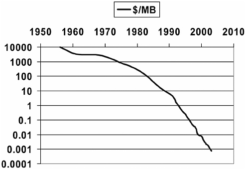
FIGURE 5.1 Decline in the price of disk space, 1950 to 2004.

disk space since the first disks in the mid-1950s, generally following the cost-performance trends of Moore’s law.

Cheaper storage led to larger and larger text collections online. Now there are many terabytes of data on the Web. These vastly larger volumes mean that precision has now become more important, since a common problem is to wade through vastly too many documents. Not surprisingly, in the mid-1980s efforts started on separating the multiple meanings of words like “bank” or “pine” and became the research area of “sense disambiguation.” 2 With sense disambiguation, it is possible to imagine searching for only one meaning of an ambiguous word, thus avoiding many erroneous retrievals.

Large-scale research on text processing took off with the availability of the TREC (Text Retrieval Evaluation Conference) data. Thanks to the National Institute of Standards and Technology, several hundred megabytes of text were provided (in each of several years) for research use. This stimulated more work on query analysis, text handling, searching

algorithms, and related areas; see the series titled TREC Conference Proceedings, edited by Donna Harmon of NIST.

Document clustering appeared as an important way to shorten long search results. Clustering enables a system to report not, say, 5000 documents but rather 10 groups of 500 documents each, and the user can then explore the group or groups that seem relevant. Salton anticipated the future possibility of such algorithms, as did others. 3 Until we got large collections, though, clustering did not find application in the document retrieval world. Now one routinely sees search engines using these techniques, and faster clustering algorithms have been developed.

Thus the algorithms explored switched from recall aids to precision aids as the quantity of available data increased. Manual thesauri, for example, have dropped out of favor for retrieval, partly because of their cost but also because their goal is to increase recall, which is not today’s problem. In terms of finding the concepts hinted at by words and phrases, our goals now are to sharpen rather than broaden these concepts: thus disambiguation and phrase matching, and not as much work on thesauri and term associations.

Again, multilingual searching started to matter, because multilingual collections became available. Multilingual research shows a more precise example of particular information resources driving research. The Canadian government made its Parliamentary proceedings (called Hansard ) available in both French and English, with paragraph-by-paragraph translation. This data stimulated a number of projects looking at how to handle bilingual material, including work on automatic alignment of the parallel texts, automatic linking of similar words in the two languages, and so on. 4

A similar effect was seen with the Brown corpus of tagged English text, where the part of speech of each word (e.g., whether a word is a noun or a verb) was identified. This produced a few years of work on algorithms that learned how to assign parts of speech to words in running text based on statistical techniques, such as the work by Garside. 5

One might see an analogy to various new fields of chemistry. The recognition that pesticides like DDT were environmental pollutants led to a new interest in biodegradability, and the Freon propellants used in aerosol cans stimulated research in reactions in the upper atmosphere. New substances stimulated a need to study reactions that previously had not been a top priority for chemistry and chemical engineering.

As storage became cheaper, image storage was now as practical as text storage had been a decade earlier. Starting in the 1980s we saw the IBM QBIC project demonstrating that something could be done to retrieve images directly, without having to index them by text words first. 6 Projects like this were stimulated by the availability of “clip art” such as the COREL image disks. Several different projects were driven by the easy access to images in this way, with technology moving on from color and texture to more accurate shape processing. At Berkeley, for example, the “Blobworld” project made major improvements in shape detection and recognition, as described in Carson et al. 7 These projects demonstrated that retrieval could be done with images as well as with words, and that properties of images could be found that were usable as concepts for searching.

Another new kind of data that became feasible to process was sound, in particular human speech. Here it was the Defense Advanced Research Projects Agency (DARPA) that took the lead, providing the SWITCH-BOARD corpus of spoken English. Again, the availability of a substantial file of tagged information helped stimulate many research projects that used this corpus and developed much of the technology that eventually went into the commercial speech recognition products we now have. As with the TREC contests, the competitions run by DARPA based on its spoken language data pushed the industry and the researchers to new advances. National needs created a new technology; one is reminded of the development of synthetic rubber during World War II or the advances in catalysis needed to make explosives during World War I.

Yet another kind of new data was geo-coded data, introducing a new set of conceptual ideas related to place. Geographical data started showing up in machine-readable form during the 1980s, especially with the release of the Dual Independent Map Encoding (DIME) files after the 1980

census and the Topologically Integrated Geographic Encoding and Referencing (TIGER) files from the 1990 census. The availability, free of charge, of a complete U.S. street map stimulated much research on systems to display maps, to give driving directions, and the like. 8 When aerial photographs also became available, there was the triumph of Microsoft’s “Terraserver,” which made it possible to look at a wide swath of the world from the sky along with correlated street and topographic maps. 9

More recently, in the 1990s, we have started to look at video search and retrieval. After all, if a CD-ROM contains about 300,000 times as many bytes per pound as a deck of punched cards, and a digitized video has about 500,000 times as many bytes per second as the ASCII script it comes from, we should be about where we were in the 1960s with video today. And indeed there are a few projects, most notably the Informedia project at Carnegie Mellon University, that experiment with video signals; they do not yet have ways of searching enormous collections, but they are developing algorithms that exploit whatever they can find in the video: scene breaks, closed-captioning, and so on.

Again, there is the problem of deducing concepts from a new kind of information. We started with the problem of words in one language needing to be combined when synonymous, picked apart when ambiguous, and moved on to detecting synonyms across multiple languages and then to concepts depicted in pictures and sounds. Now we see research such as that by Jezekiel Ben-Arie associating words like “run” or “hop” with video images of people doing those actions. In the same way we get again new chemistry when molecules like “buckyballs” are created and stimulate new theoretical and reaction studies.

Defining concepts for search can be extremely difficult. For example, despite our abilities to parse and define every item in a computer language, we have made no progress on retrieval of software; people looking for search or sort routines depend on metadata or comments. Some areas seem more flexible than others: text and naturalistic photograph processing software tends to be very general, while software to handle CAD diagrams and maps tends to be more specific. Algorithms are sometimes portable; both speech processing and image processing need Fourier transforms, but the literature is less connected than one might like (partly

because of the difference between one-dimensional and two-dimensional transforms).

There are many other examples of interesting computer science research stimulated by the availability of particular kinds of information. Work on string matching today is often driven by the need to align sequences in either protein or DNA data banks. Work on image analysis is heavily influenced by the need to deal with medical radiographs. And there are many other interesting projects specifically linked to an individual data source. Among examples:

The British Library scanning of the original manuscript of Beowulf in collaboration with the University of Kentucky, working on image enhancement until the result of the scanning is better than reading the original;

The Perseus project, demonstrating the educational applications possible because of the earlier Thesaurus Linguae Graecae project, which digitized all the classical Greek authors;

The work in astronomical analysis stimulated by the Sloan Digital Sky Survey;

The creation of the field of “forensic paleontology” at the University of Texas as a result of doing MRI scans of fossil bones;

And, of course, the enormous amount of work on search engines stimulated by the Web.

When one of these fields takes off, and we find wide usage of some online resource, it benefits society. Every university library gained readers as their catalogs went online and became accessible to students in their dorm rooms. Third World researchers can now access large amounts of technical content their libraries could rarely acquire in the past.

In computer science, and in chemistry, there is a tension between the algorithm/reaction and the data/substance. For example, should one look up an answer or compute it? Once upon a time logarithms were looked up in tables; today we also compute them on demand. Melting points and other physical properties of chemical substances are looked up in tables; perhaps with enough quantum mechanical calculation we could predict them, but it’s impractical for most materials. Predicting tomorrow’s weather might seem a difficult choice. One approach is to measure the current conditions, take some equations that model the atmosphere, and calculate forward a day. Another is to measure the current conditions, look in a big database for the previous day most similar to today, and then take the day after that one as the best prediction for tomorrow. However, so far the meteorologists feel that calculation is better. Another complicated example is chess: given the time pressure of chess tournaments

against speed and storage available in computers, chess programs do the opening and the endgame by looking in tables of old data and calculate for the middle game.

To conclude, a recipe for stimulating advances in computer science is to make some data available and let people experiment with it. With the incredibly cheap disks and scanners available today, this should be easier than ever. Unfortunately, what we gain with technology we are losing to law and economics. Many large databases are protected by copyright; few motion pictures, for example, are old enough to have gone out of copyright. Content owners generally refuse to grant permission for wide use of their material, whether out of greed or fear: they may have figured out how to get rich off their files of information or they may be afraid that somebody else might have. Similarly it is hard to get permission to digitize in-copyright books, no matter how long they have been out of print. Jim Gray once said to me, “May all your problems be technical.” In the 1960s I was paying people to key in aeronautical abstracts. It never occurred to us that we should be asking permission of the journals involved (I think what we did would qualify as fair use, but we didn’t even think about it). Today I could scan such things much more easily, but I would not be able to get permission. Am I better off or worse off?

There are now some 22 million chemical substances in the Chemical Abstracts Service Registry and 7 million reactions. New substances continue to intrigue chemists and cause research on new reactions, with of course enormous interest in biochemistry both for medicine and agriculture. Similarly, we keep adding data to the Web, and new kinds of information (photographs of dolphins, biological flora, and countless other things) can push computer scientists to new algorithms. In both cases, synthesis of specific instances into concepts is a crucial problem. As we see more and more kinds of data, we learn more about how to extract meaning from it, and how to present it, and we develop a need for new algorithms to implement this knowledge. As the data gets bigger, we learn more about optimization. As it gets more complex, we learn more about representation. And as it gets more useful, we learn more about visualization and interfaces, and we provide better service to society.

HISTORY AND THE FUNDAMENTALS OF COMPUTER SCIENCE

Edward L. Ayers, University of Virginia

We might begin with a thought experiment: What is history? Many people, I’ve discovered, think of it as books and the things in books. That’s certainly the explicit form in which we usually confront history. Others, thinking less literally, might think of history as stories about the past; that would open us to oral history, family lore, movies, novels, and the other forms in which we get most of our history.

All these images are wrong, of course, in the same way that images of atoms as little solar systems are wrong, or pictures of evolution as profiles of ever taller and more upright apes and people are wrong. They are all models, radically simplified, that allow us to think about such things in the exceedingly small amounts of time that we allot to these topics.

The same is true for history, which is easiest to envision as technological progress, say, or westward expansion, of the emergence of freedom—or of increasing alienation, exploitation of the environment, or the growth of intrusive government.

Those of us who think about specific aspects of society or nature for a living, of course, are never satisfied with the stories that suit the purposes of everyone else so well.

We are troubled by all the things that don’t fit, all the anomalies, variance, and loose ends. We demand more complex measurement, description, and fewer smoothing metaphors and lowest common denominators.

Thus, to scientists, atoms appear as clouds of probability; evolution appears as a branching, labyrinthine bush in which some branches die out and others diversify. It can certainly be argued that past human experience is as complex as anything in nature and likely much more so, if by complexity we mean numbers of components, variability of possibilities, and unpredictability of outcomes.

Yet our means of conveying that complexity remain distinctly analog: the story, the metaphor, the generalization. Stories can be wonderfully complex, of course, but they are complex in specific ways: of implication, suggestion, evocation. That’s what people love and what they remember.

But maybe there is a different way of thinking about the past: as information. In fact, information is all we have. Studying the past is like studying scientific processes for which you have the data but cannot run the experiment again, in which there is no control, and in which you can never see the actual process you are describing and analyzing. All we have is information in various forms: words in great abundance, billions of numbers, millions of images, some sounds and buildings, artifacts.

The historian’s goal, it seems to me, should be to account for as much of the complexity embedded in that information as we can. That, it appears, is what scientists do, and it has served them well.

And how has science accounted for ever-increasing amounts of complexity in the information they use? Through ever more sophisticated instruments. The connection between computer science and history could be analogous to that between telescopes and stars, microscopes and cells. We could be on the cusp of a new understanding of the patterns of complexity in human behavior of the past.

The problem may be that there is too much complexity in that past, or too much static, or too much silence. In the sciences, we’ve learned how to filter, infer, use indirect evidence, and fill in the gaps, but we have a much more literal approach to the human past.

We have turned to computer science for tasks of more elaborate description, classification, representation. The digital archive my colleagues and I have built, the Valley of the Shadow Project, permits the manipulation of millions of discrete pieces of evidence about two communities in the era of the American Civil War. It uses sorting mechanisms, hypertextual display, animation, and the like to allow people to handle the evidence of this part of the past for themselves. This isn’t cutting-edge computer science, of course, but it’s darned hard and deeply disconcerting to some, for it seems to abdicate responsibility, to undermine authority, to subvert narrative, to challenge story.

Now, we’re trying to take this work to the next stage, to analysis. We have composed a journal article that employs an array of technologies, especially geographic information systems and statistical analysis in the creation of the evidence. The article presents its argument, evidence, and historiographical context as a complex textual, tabular, and graphical representation. XML offers a powerful means to structure text and XSL an even more powerful means to transform it and manipulate its presentation. The text is divided into sections called “statements,” each supported with “explanation.” Each explanation, in turn, is supported by evidence and connected to relevant historiography.

Linkages, forward and backward, between evidence and narrative are central. The historiography can be automatically sorted by author, date, or title; the evidence can be arranged by date, topic, or type. Both evidence and historiographical entries are linked to the places in the analysis where they are invoked. The article is meant to be used online, but it can be printed in a fixed format with all the limitations and advantages of print.

So, what are the implications of thinking of the past in the hardheaded sense of admitting that all we really have of the past is information? One implication might be great humility, since all we have for most

of the past are the fossils of former human experience, words frozen in ink and images frozen in line and color. Another implication might be hubris: if we suddenly have powerful new instruments, might we be on the threshold of a revolution in our understanding of the past? We’ve been there before.

A connection between history and social science was tried before, during the first days of accessible computers. Historians taught themselves statistical methods and even programming languages so that they could adopt the techniques, models, and insights of sociology and political science. In the 1950s and 1960s the creators of the new political history called on historians to emulate the precision, explicitness, replicability, and inclusivity of the quantitative social sciences. For two decades that quantitative history flourished, promising to revolutionize the field. And to a considerable extent it did: it changed our ideas of social mobility, political identification, family formation, patterns of crime, economic growth, and the consequences of ethnic identity. It explicitly linked the past to the present and held out a history of obvious and immediate use.

But that quantitative social science history collapsed suddenly, the victim of its own inflated claims, limited method and machinery, and changing academic fashion. By the mid-1980s, history, along with many of the humanities and social sciences, had taken the linguistic turn. Rather than software manuals and codebooks, graduate students carried books of French philosophy and German literary interpretation. The social science of choice shifted from sociology to anthropology; texts replaced tables. A new generation defined itself in opposition to social scientific methods just as energetically as an earlier generation had seen in those methods the best means of writing a truly democratic history. The first computer revolution largely failed.

The first effort at that history fell into decline in part because historians could not abide the distance between their most deeply held beliefs and what the statistical machinery permitted, the abstraction it imposed. History has traditionally been built around contingency and particularity, but the most powerful tools of statistics are built on sampling and extrapolation, on generalization and tendency. Older forms of social history talked about vague and sometimes dubious classifications in part because that was what the older technology of tabulation permitted us to see. It has become increasingly clear across the social sciences that such flat ways of describing social life are inadequate; satisfying explanations must be dynamic, interactive, reflexive, and subtle, refusing to reify structures of social life or culture. The new technology permits a new cross-fertilization.

Ironically, social science history faded just as computers became widely available, just as new kinds of social science history became feasible. No longer is there any need for white-coated attendants at huge mainframes

and expensive proprietary software. Rather than reducing people to rows and columns, searchable databases now permit researchers to maintain the identities of individuals in those databases and to represent entire populations rather than samples. Moreover, the record can now include things social science history could only imagine before the Web: completely indexed newspapers, with the original readable on the screen; completely searchable letters and diaries by the thousands; and interactive maps with all property holders identified and linked to other records. Visualization of patterns in the data, moreover, far outstrips the possibilities of numerical calculation alone. Manipulable histograms, maps, and time lines promise a social history that is simultaneously sophisticated and accessible. We have what earlier generations of social science historians dreamed of: a fast and widely accessible network linked to cheap and powerful computers running common software with well-established standards for the handling of numbers, texts, and images. New possibilities of collaboration and cumulative research beckon. Perhaps the time is right to reclaim a worthy vision of a disciplined and explicit social scientific history that we abandoned too soon.

What does this have to do with computer science? Everything, it seems to me. If you want hard problems, historians have them. And what’s the hardest problem of all right now? The capture of the very information that is history. Can computer science imagine ways to capture historical information more efficiently? Can it offer ways to work with the spotty, broken, dirty, contradictory, nonstandardized information we work with?

The second hard problem is the integration of this disparate evidence in time and space, offering new precision, clarity, and verifiability, as well as opening new questions and new ways of answering them.

If we can think of these ways, then we face virtually limitless possibilities. Is there a more fundamental challenge or opportunity for computer science than helping us to figure out human society over human time?

This page intentionally left blank.

Computer Science: Reflections on the Field, Reflections from the Field provides a concise characterization of key ideas that lie at the core of computer science (CS) research. The book offers a description of CS research recognizing the richness and diversity of the field. It brings together two dozen essays on diverse aspects of CS research, their motivation and results. By describing in accessible form computer science’s intellectual character, and by conveying a sense of its vibrancy through a set of examples, the book aims to prepare readers for what the future might hold and help to inspire CS researchers in its creation.

Welcome to OpenBook!

You're looking at OpenBook, NAP.edu's online reading room since 1999. Based on feedback from you, our users, we've made some improvements that make it easier than ever to read thousands of publications on our website.

Do you want to take a quick tour of the OpenBook's features?

Show this book's table of contents , where you can jump to any chapter by name.

...or use these buttons to go back to the previous chapter or skip to the next one.

Jump up to the previous page or down to the next one. Also, you can type in a page number and press Enter to go directly to that page in the book.

Switch between the Original Pages , where you can read the report as it appeared in print, and Text Pages for the web version, where you can highlight and search the text.

To search the entire text of this book, type in your search term here and press Enter .

Share a link to this book page on your preferred social network or via email.

View our suggested citation for this chapter.

Ready to take your reading offline? Click here to buy this book in print or download it as a free PDF, if available.

Get Email Updates

Do you enjoy reading reports from the Academies online for free ? Sign up for email notifications and we'll let you know about new publications in your areas of interest when they're released.

Talk to our experts

1800-120-456-456

• Introduction to Data Representation
• Computer Science

About Data Representation

Data can be anything, including a number, a name, musical notes, or the colour of an image. The way that we stored, processed, and transmitted data is referred to as data representation. We can use any device, including computers, smartphones, and iPads, to store data in digital format. The stored data is handled by electronic circuitry. A bit is a 0 or 1 used in digital data representation.

Data Representation Techniques

Classification of Computers

Computer scans are classified broadly based on their speed and computing power.

1. Microcomputers or PCs (Personal Computers): It is a single-user computer system with a medium-power microprocessor. It is referred to as a computer with a microprocessor as its central processing unit.

Microcomputer

2. Mini-Computer: It is a multi-user computer system that can support hundreds of users at the same time.

Types of Mini Computers

3. Mainframe Computer: It is a multi-user computer system that can support hundreds of users at the same time. Software technology is distinct from minicomputer technology.

Mainframe Computer

4. Super-Computer: With the ability to process hundreds of millions of instructions per second, it is a very quick computer. They  are used for specialised applications requiring enormous amounts of mathematical computations, but they are very expensive.

Supercomputer

Types of Computer Number System

Every value saved to or obtained from computer memory uses a specific number system, which is the method used to represent numbers in the computer system architecture. One needs to be familiar with number systems in order to read computer language or interact with the system. 

Types of Number System

1. Binary Number System 

There are only two digits in a binary number system: 0 and 1. In this number system, 0 and 1 stand in for every number (value). Because the binary number system only has two digits, its base is 2.

A bit is another name for each binary digit. The binary number system is also a positional value system, where each digit's value is expressed in powers of 2.

Characteristics of Binary Number System

The following are the primary characteristics of the binary system:

It only has two digits, zero and one.

Depending on its position, each digit has a different value.

Each position has the same value as a base power of two.

Because computers work with internal voltage drops, it is used in all types of computers.

Binary Number System

2. Decimal Number System

The decimal number system is a base ten number system with ten digits ranging from 0 to 9. This means that these ten digits can represent any numerical quantity. A positional value system is also a decimal number system. This means that the value of digits will be determined by their position. 

Characteristics of Decimal Number System

Ten units of a given order equal one unit of the higher order, making it a decimal system.

The number 10 serves as the foundation for the decimal number system.

The value of each digit or number will depend on where it is located within the numeric figure because it is a positional system.

The value of this number results from multiplying all the digits by each power.

Decimal Number System

Decimal Binary Conversion Table

3. octal number system.

There are only eight (8) digits in the octal number system, from 0 to 7. In this number system, each number (value) is represented by the digits 0, 1, 2, 3,4,5,6, and 7. Since the octal number system only has 8 digits, its base is 8.

Characteristics of Octal Number System:

Contains eight digits: 0,1,2,3,4,5,6,7.

Also known as the base 8 number system.

Each octal number position represents a 0 power of the base (8). 

An octal number's last position corresponds to an x power of the base (8).

Octal Number System

4. Hexadecimal Number System

There are sixteen (16) alphanumeric values in the hexadecimal number system, ranging from 0 to 9 and A to F. In this number system, each number (value) is represented by 0, 1, 2, 3, 5, 6, 7, 8, 9, A, B, C, D, E, and F. Because the hexadecimal number system has 16 alphanumeric values, its base is 16. Here, the numbers are A = 10, B = 11, C = 12, D = 13, E = 14, and F = 15.

Characteristics of Hexadecimal Number System:

A system of positional numbers.

Has 16 symbols or digits overall (0, 1, 2, 3, 4, 5, 6, 7, 8, 9, A, B, C, D, E, F). Its base is, therefore, 16.

Decimal values 10, 11, 12, 13, 14, and 15 are represented by the letters A, B, C, D, E, and F, respectively.

A single digit may have a maximum value of 15. 

Each digit position corresponds to a different base power (16).

Since there are only 16 digits, any hexadecimal number can be represented in binary with 4 bits.

Hexadecimal Number System

So, we've seen how to convert decimals and use the Number System to communicate with a computer. The full character set of the English language, which includes all alphabets, punctuation marks, mathematical operators, special symbols, etc., must be supported by the computer in addition to numerical data. 

Learning By Doing

Choose the correct answer:.

1. Which computer is the largest in terms of size?

Minicomputer

Micro Computer

2. The binary number 11011001 is converted to what decimal value?

Solved Questions

1. Give some examples where Supercomputers are used.

Ans: Weather Prediction, Scientific simulations, graphics, fluid dynamic calculations, Nuclear energy research, electronic engineering and analysis of geological data.

2. Which of these is the most costly?

Mainframe computer

Ans: C) Supercomputer

FAQs on Introduction to Data Representation

1. What is the distinction between the Hexadecimal and Octal Number System?

The octal number system is a base-8 number system in which the digits 0 through 7 are used to represent numbers. The hexadecimal number system is a base-16 number system that employs the digits 0 through 9 as well as the letters A through F to represent numbers.

2. What is the smallest data representation?

The smallest data storage unit in a computer's memory is called a BYTE, which comprises 8 BITS.

3. What is the largest data unit?

The largest commonly available data storage unit is a terabyte or TB. A terabyte equals 1,000 gigabytes, while a tebibyte equals 1,024 gibibytes.

• Even more »

Account Options

• Try the new Google Books
• Advanced Book Search
• Bentham Science Publishers
• Barnes&Noble.com
• Books-A-Million
• Find in a library
• All sellers  »

Get Textbooks on Google Play

Rent and save from the world's largest eBookstore. Read, highlight, and take notes, across web, tablet, and phone.

Go to Google Play Now »

Selected pages

Other editions - View all

Common terms and phrases, bibliographic information.

• Computer Concepts Tutorial
• Computer Concepts - Home
• Introduction to Computer
• Introduction to GUI based OS
• Elements of Word Processing
• Spread Sheet
• Introduction to Internet, WWW, Browsers
• Communication & Collaboration
• Application of Presentations
• Application of Digital Financial Services
• Computer Concepts Resources
• Computer Concepts - Quick Guide
• Computer Concepts - Useful Resources
• Computer Concepts - Discussion
• Selected Reading
• UPSC IAS Exams Notes
• Developer's Best Practices
• Questions and Answers
• Effective Resume Writing
• HR Interview Questions
• Computer Glossary

Representation of Data/Information

Computer does not understand human language. Any data, viz., letters, symbols, pictures, audio, videos, etc., fed to computer should be converted to machine language first. Computers represent data in the following three forms −

Number System

We are introduced to concept of numbers from a very early age. To a computer, everything is a number, i.e., alphabets, pictures, sounds, etc., are numbers. Number system is categorized into four types −

Binary number system consists of only two values, either 0 or 1

Octal number system represents values in 8 digits.

Decimal number system represents values in 10 digits.

Hexadecimal number system represents values in 16 digits.

Bits and Bytes

Bits − A bit is a smallest possible unit of data that a computer can recognize or use. Computer usually uses bits in groups.

Bytes − group of eight bits is called a byte. Half a byte is called a nibble.

The following table shows conversion of Bits and Bytes −

Text code is format used commonly to represent alphabets, punctuation marks and other symbols. Four most popular text code systems are −

Extended ASCII

Extended Binary Coded Decimal Interchange Code is an 8-bit code that defines 256 symbols. Given below is the EBCDIC Tabular column

American Standard Code for Information Interchange is an 8-bit code that specifies character values from 0 to 127.

ASCII Tabular column

Extended American Standard Code for Information Interchange is an 8-bit code that specifies character values from 128 to 255.

Extended ASCII Tabular column

Unicode Worldwide Character Standard uses 4 to 32 bits to represent letters, numbers and symbol.

Unicode Tabular Column

If you're seeing this message, it means we're having trouble loading external resources on our website.

If you're behind a web filter, please make sure that the domains *.kastatic.org and *.kasandbox.org are unblocked.

To log in and use all the features of Khan Academy, please enable JavaScript in your browser.

Praxis Core Math

Course: praxis core math   >   unit 1, data representations | lesson.

• Data representations | Worked example
• Center and spread | Lesson
• Center and spread | Worked example
• Random sampling | Lesson
• Random sampling | Worked example
• Scatterplots | Lesson
• Scatterplots | Worked example
• Interpreting linear models | Lesson
• Interpreting linear models | Worked example
• Correlation and Causation | Lesson
• Correlation and causation | Worked example
• Probability | Lesson
• Probability | Worked example

What are data representations?

• How much of the data falls within a specified category or range of values?
• What is a typical value of the data?
• How much spread is in the data?
• Is there a trend in the data over time?
• Is there a relationship between two variables?

What skills are tested?

• Matching a data set to its graphical representation
• Matching a graphical representation to a description
• Using data representations to solve problems

How are qualitative data displayed?

• A table summarizes the data using rows and columns. Each column contains data for a single variable, and a basic table contains one column for the qualitative variable and one for the quantitative variable. Each row contains a category of the qualitative variable and the corresponding value of the quantitative variable. [Example]
• A vertical bar chart lists the categories of the qualitative variable along a horizontal axis and uses the heights of the bars on the vertical axis to show the values of the quantitative variable. A horizontal bar chart lists the categories along the vertical axis and uses the lengths of the bars on the horizontal axis to show the values of the quantitative variable. This display draws attention to how the categories rank according to the amount of data within each. [Example]
• A pictograph is like a horizontal bar chart but uses pictures instead of the lengths of bars to represent the values of the quantitative variable. Each picture represents a certain quantity, and each category can have multiple pictures. Pictographs are visually interesting, but require us to use the legend to convert the number of pictures to quantitative values. [Example]
• A circle graph (or pie chart) is a circle that is divided into as many sections as there are categories of the qualitative variable. The area of each section represents, for each category, the value of the quantitative data as a fraction of the sum of values. The fractions sum to 1 ‍   . Sometimes the section labels include both the category and the associated value or percent value for that category. [Example]

How are quantitative data displayed?

• Dotplots use one dot for each data point. The dots are plotted above their corresponding values on a number line. The number of dots above each specific value represents the count of that value. Dotplots show the value of each data point and are practical for small data sets. [Example]
• Histograms divide the horizontal axis into equal-sized intervals and use the heights of the bars to show the count or percent of data within each interval. By convention, each interval includes the lower boundary but not the upper one. Histograms show only totals for the intervals, not specific data points. [Example]

How are trends over time displayed?

How are relationships between variables displayed.

• (Choice A)   A
• (Choice B)   B
• (Choice C)   C
• (Choice D)   D
• (Choice E)   E
• Your answer should be
• an integer, like 6 ‍  
• a simplified proper fraction, like 3 / 5 ‍  
• a simplified improper fraction, like 7 / 4 ‍  
• a mixed number, like 1   3 / 4 ‍  
• an exact decimal, like 0.75 ‍  
• a multiple of pi, like 12   pi ‍   or 2 / 3   pi ‍  
• a proper fraction, like 1 / 2 ‍   or 6 / 10 ‍  
• an improper fraction, like 10 / 7 ‍   or 14 / 8 ‍  

Things to remember

• When matching data to a representation, check that the values are graphed accurately for all categories.
• When reporting data counts or fractions, be clear whether a question asks about data within a single category or a comparison between categories.
• When finding the number or fraction of the data meeting a criteria, watch for key words such as or , and , less than , and more than .

Want to join the conversation?

• Upvote Button navigates to signup page
• Downvote Button navigates to signup page
• Flag Button navigates to signup page

Computer Network

• Operating Systems
• Computer Fundamentals
• Interview Q

Physical Layer

Data link layer, network layer, routing algorithm, transport layer, application layer, application protocols, network security.

Interview Questions

• Send your Feedback to [email protected]

Help Others, Please Share

Learn Latest Tutorials

Transact-SQL

Reinforcement Learning

R Programming

React Native

Python Design Patterns

Python Pillow

Python Turtle

Preparation

Verbal Ability

Company Questions

Trending Technologies

Artificial Intelligence

Cloud Computing

Data Science

Machine Learning

B.Tech / MCA

Data Structures

Operating System

Compiler Design

Computer Organization

Discrete Mathematics

Ethical Hacking

Computer Graphics

Software Engineering

Web Technology

Cyber Security

C Programming

Control System

Data Mining

Data Warehouse

Green Chemistry

An interpretable 3d multi-hierarchical representation-based deep neural network for environmental, health and safety properties prediction of organic solvents †.

* Corresponding authors

a School of Chemistry and Chemical Engineering, Chongqing University, Chongqing 400044, China E-mail: [email protected]

b School of Chemistry and Chemical Engineering, Chongqing University of Science and Technology, Chongqing 401331, China E-mail: [email protected]

c School of Chemistry and Chemical Engineering, Hubei Key Laboratory of Coal Conversion and New Carbon Materials, Wuhan University of Science and Technology, Wuhan 430081, Hubei, China

The interpretability and accuracy of deep-learning-based predictive models play a pivotal role in accelerating computer-aided green product design considering environmental, health, and safety (EH&S) impacts. Recently, molecular graph-based hybrid representation methods have demonstrated comparable or superior abilities to other molecular representations. However, existing molecular graph-based hybrid representation methods incorporate only 2D-based atom-level, bond-level, or molecule-level features while neglecting the molecular geometry, also known as 3D spatial structure information, which is crucial for determining molecular properties. Moreover, existing molecular graph-based hybrid representations lack consideration of knowledge in the chemistry domain, which can improve the interpretability of the predictive models. To this end, a 3D multi-hierarchical representation-based deep neural network (3D-MrDNN) architecture, simultaneously integrating directed message passing neural network learned representation, chemically synthesizable fragment features, and molecular 3D spatial information, is established for the prediction of EH&S properties. The results of predictive performance and ablation studies indicate that the proposed model exhibits decent predictive ability for EH&S properties. Chemically synthesizable fragments are utilized to integrate chemical knowledge into the proposed 3D-MrDNN architecture, the interpretability of which enables chemists to find the key molecular fragments for designing target products with better EH&S performance.

Supplementary files

• Supplementary information XLSX (697K)

Article information

Download citation, permissions.

An interpretable 3D multi-hierarchical representation-based deep neural network for environmental, health and safety properties prediction of organic solvents

J. Zhang, Q. Wang, Y. Lei and W. Shen, Green Chem. , 2024, Advance Article , DOI: 10.1039/D3GC04801B

To request permission to reproduce material from this article, please go to the Copyright Clearance Center request page .

If you are an author contributing to an RSC publication, you do not need to request permission provided correct acknowledgement is given.

If you are the author of this article, you do not need to request permission to reproduce figures and diagrams provided correct acknowledgement is given. If you want to reproduce the whole article in a third-party publication (excluding your thesis/dissertation for which permission is not required) please go to the Copyright Clearance Center request page .

Read more about how to correctly acknowledge RSC content .

Social activity

Search articles by author.

This article has not yet been cited.

Advertisements

Help | Advanced Search

Computer Science > Computer Vision and Pattern Recognition

Title: dynamic graph representation with knowledge-aware attention for histopathology whole slide image analysis.

Abstract: Histopathological whole slide images (WSIs) classification has become a foundation task in medical microscopic imaging processing. Prevailing approaches involve learning WSIs as instance-bag representations, emphasizing significant instances but struggling to capture the interactions between instances. Additionally, conventional graph representation methods utilize explicit spatial positions to construct topological structures but restrict the flexible interaction capabilities between instances at arbitrary locations, particularly when spatially distant. In response, we propose a novel dynamic graph representation algorithm that conceptualizes WSIs as a form of the knowledge graph structure. Specifically, we dynamically construct neighbors and directed edge embeddings based on the head and tail relationships between instances. Then, we devise a knowledge-aware attention mechanism that can update the head node features by learning the joint attention score of each neighbor and edge. Finally, we obtain a graph-level embedding through the global pooling process of the updated head, serving as an implicit representation for the WSI classification. Our end-to-end graph representation learning approach has outperformed the state-of-the-art WSI analysis methods on three TCGA benchmark datasets and in-house test sets. Our code is available at this https URL .

Submission history

Access paper:.

• Download PDF
• HTML (experimental)
• Other Formats

References & Citations

• Google Scholar
• Semantic Scholar

BibTeX formatted citation

Bibliographic and Citation Tools

Code, data and media associated with this article, recommenders and search tools.

• Institution

arXivLabs: experimental projects with community collaborators

arXivLabs is a framework that allows collaborators to develop and share new arXiv features directly on our website.

Both individuals and organizations that work with arXivLabs have embraced and accepted our values of openness, community, excellence, and user data privacy. arXiv is committed to these values and only works with partners that adhere to them.

Have an idea for a project that will add value for arXiv's community? Learn more about arXivLabs .