

User Preferences
Content preview.
Arcu felis bibendum ut tristique et egestas quis:
- Ut enim ad minim veniam, quis nostrud exercitation ullamco laboris
- Duis aute irure dolor in reprehenderit in voluptate
- Excepteur sint occaecat cupidatat non proident
Keyboard Shortcuts
S.3 hypothesis testing.
In reviewing hypothesis tests, we start first with the general idea. Then, we keep returning to the basic procedures of hypothesis testing, each time adding a little more detail.
The general idea of hypothesis testing involves:
- Making an initial assumption.
- Collecting evidence (data).
- Based on the available evidence (data), deciding whether to reject or not reject the initial assumption.
Every hypothesis test — regardless of the population parameter involved — requires the above three steps.
Example S.3.1
Is normal body temperature really 98.6 degrees f section .
Consider the population of many, many adults. A researcher hypothesized that the average adult body temperature is lower than the often-advertised 98.6 degrees F. That is, the researcher wants an answer to the question: "Is the average adult body temperature 98.6 degrees? Or is it lower?" To answer his research question, the researcher starts by assuming that the average adult body temperature was 98.6 degrees F.
Then, the researcher went out and tried to find evidence that refutes his initial assumption. In doing so, he selects a random sample of 130 adults. The average body temperature of the 130 sampled adults is 98.25 degrees.
Then, the researcher uses the data he collected to make a decision about his initial assumption. It is either likely or unlikely that the researcher would collect the evidence he did given his initial assumption that the average adult body temperature is 98.6 degrees:
- If it is likely , then the researcher does not reject his initial assumption that the average adult body temperature is 98.6 degrees. There is not enough evidence to do otherwise.
- either the researcher's initial assumption is correct and he experienced a very unusual event;
- or the researcher's initial assumption is incorrect.
In statistics, we generally don't make claims that require us to believe that a very unusual event happened. That is, in the practice of statistics, if the evidence (data) we collected is unlikely in light of the initial assumption, then we reject our initial assumption.
Example S.3.2
Criminal trial analogy section .
One place where you can consistently see the general idea of hypothesis testing in action is in criminal trials held in the United States. Our criminal justice system assumes "the defendant is innocent until proven guilty." That is, our initial assumption is that the defendant is innocent.
In the practice of statistics, we make our initial assumption when we state our two competing hypotheses -- the null hypothesis ( H 0 ) and the alternative hypothesis ( H A ). Here, our hypotheses are:
- H 0 : Defendant is not guilty (innocent)
- H A : Defendant is guilty
In statistics, we always assume the null hypothesis is true . That is, the null hypothesis is always our initial assumption.
The prosecution team then collects evidence — such as finger prints, blood spots, hair samples, carpet fibers, shoe prints, ransom notes, and handwriting samples — with the hopes of finding "sufficient evidence" to make the assumption of innocence refutable.
In statistics, the data are the evidence.
The jury then makes a decision based on the available evidence:
- If the jury finds sufficient evidence — beyond a reasonable doubt — to make the assumption of innocence refutable, the jury rejects the null hypothesis and deems the defendant guilty. We behave as if the defendant is guilty.
- If there is insufficient evidence, then the jury does not reject the null hypothesis . We behave as if the defendant is innocent.
In statistics, we always make one of two decisions. We either "reject the null hypothesis" or we "fail to reject the null hypothesis."
Errors in Hypothesis Testing Section
Did you notice the use of the phrase "behave as if" in the previous discussion? We "behave as if" the defendant is guilty; we do not "prove" that the defendant is guilty. And, we "behave as if" the defendant is innocent; we do not "prove" that the defendant is innocent.
This is a very important distinction! We make our decision based on evidence not on 100% guaranteed proof. Again:
- If we reject the null hypothesis, we do not prove that the alternative hypothesis is true.
- If we do not reject the null hypothesis, we do not prove that the null hypothesis is true.
We merely state that there is enough evidence to behave one way or the other. This is always true in statistics! Because of this, whatever the decision, there is always a chance that we made an error .
Let's review the two types of errors that can be made in criminal trials:
Table S.3.2 shows how this corresponds to the two types of errors in hypothesis testing.
Note that, in statistics, we call the two types of errors by two different names -- one is called a "Type I error," and the other is called a "Type II error." Here are the formal definitions of the two types of errors:
There is always a chance of making one of these errors. But, a good scientific study will minimize the chance of doing so!
Making the Decision Section
Recall that it is either likely or unlikely that we would observe the evidence we did given our initial assumption. If it is likely , we do not reject the null hypothesis. If it is unlikely , then we reject the null hypothesis in favor of the alternative hypothesis. Effectively, then, making the decision reduces to determining "likely" or "unlikely."
In statistics, there are two ways to determine whether the evidence is likely or unlikely given the initial assumption:
- We could take the " critical value approach " (favored in many of the older textbooks).
- Or, we could take the " P -value approach " (what is used most often in research, journal articles, and statistical software).
In the next two sections, we review the procedures behind each of these two approaches. To make our review concrete, let's imagine that μ is the average grade point average of all American students who major in mathematics. We first review the critical value approach for conducting each of the following three hypothesis tests about the population mean $\mu$:
In Practice
- We would want to conduct the first hypothesis test if we were interested in concluding that the average grade point average of the group is more than 3.
- We would want to conduct the second hypothesis test if we were interested in concluding that the average grade point average of the group is less than 3.
- And, we would want to conduct the third hypothesis test if we were only interested in concluding that the average grade point average of the group differs from 3 (without caring whether it is more or less than 3).
Upon completing the review of the critical value approach, we review the P -value approach for conducting each of the above three hypothesis tests about the population mean \(\mu\). The procedures that we review here for both approaches easily extend to hypothesis tests about any other population parameter.
- Search Search Please fill out this field.
- Fundamental Analysis
Hypothesis to Be Tested: Definition and 4 Steps for Testing with Example
:max_bytes(150000):strip_icc():format(webp)/ChristinaMajaski-5c9433ea46e0fb0001d880b1.jpeg "concept of hypothesis testing")
What Is Hypothesis Testing?
Hypothesis testing, sometimes called significance testing, is an act in statistics whereby an analyst tests an assumption regarding a population parameter. The methodology employed by the analyst depends on the nature of the data used and the reason for the analysis.
Hypothesis testing is used to assess the plausibility of a hypothesis by using sample data. Such data may come from a larger population, or from a data-generating process. The word "population" will be used for both of these cases in the following descriptions.
Key Takeaways
- Hypothesis testing is used to assess the plausibility of a hypothesis by using sample data.
- The test provides evidence concerning the plausibility of the hypothesis, given the data.
- Statistical analysts test a hypothesis by measuring and examining a random sample of the population being analyzed.
- The four steps of hypothesis testing include stating the hypotheses, formulating an analysis plan, analyzing the sample data, and analyzing the result.
How Hypothesis Testing Works
In hypothesis testing, an analyst tests a statistical sample, with the goal of providing evidence on the plausibility of the null hypothesis.
Statistical analysts test a hypothesis by measuring and examining a random sample of the population being analyzed. All analysts use a random population sample to test two different hypotheses: the null hypothesis and the alternative hypothesis.
The null hypothesis is usually a hypothesis of equality between population parameters; e.g., a null hypothesis may state that the population mean return is equal to zero. The alternative hypothesis is effectively the opposite of a null hypothesis (e.g., the population mean return is not equal to zero). Thus, they are mutually exclusive , and only one can be true. However, one of the two hypotheses will always be true.
The null hypothesis is a statement about a population parameter, such as the population mean, that is assumed to be true.
4 Steps of Hypothesis Testing
All hypotheses are tested using a four-step process:
- The first step is for the analyst to state the hypotheses.
- The second step is to formulate an analysis plan, which outlines how the data will be evaluated.
- The third step is to carry out the plan and analyze the sample data.
- The final step is to analyze the results and either reject the null hypothesis, or state that the null hypothesis is plausible, given the data.
Real-World Example of Hypothesis Testing
If, for example, a person wants to test that a penny has exactly a 50% chance of landing on heads, the null hypothesis would be that 50% is correct, and the alternative hypothesis would be that 50% is not correct.
Mathematically, the null hypothesis would be represented as Ho: P = 0.5. The alternative hypothesis would be denoted as "Ha" and be identical to the null hypothesis, except with the equal sign struck-through, meaning that it does not equal 50%.
A random sample of 100 coin flips is taken, and the null hypothesis is then tested. If it is found that the 100 coin flips were distributed as 40 heads and 60 tails, the analyst would assume that a penny does not have a 50% chance of landing on heads and would reject the null hypothesis and accept the alternative hypothesis.
If, on the other hand, there were 48 heads and 52 tails, then it is plausible that the coin could be fair and still produce such a result. In cases such as this where the null hypothesis is "accepted," the analyst states that the difference between the expected results (50 heads and 50 tails) and the observed results (48 heads and 52 tails) is "explainable by chance alone."
Some staticians attribute the first hypothesis tests to satirical writer John Arbuthnot in 1710, who studied male and female births in England after observing that in nearly every year, male births exceeded female births by a slight proportion. Arbuthnot calculated that the probability of this happening by chance was small, and therefore it was due to “divine providence.”
What is Hypothesis Testing?
Hypothesis testing refers to a process used by analysts to assess the plausibility of a hypothesis by using sample data. In hypothesis testing, statisticians formulate two hypotheses: the null hypothesis and the alternative hypothesis. A null hypothesis determines there is no difference between two groups or conditions, while the alternative hypothesis determines that there is a difference. Researchers evaluate the statistical significance of the test based on the probability that the null hypothesis is true.
What are the Four Key Steps Involved in Hypothesis Testing?
Hypothesis testing begins with an analyst stating two hypotheses, with only one that can be right. The analyst then formulates an analysis plan, which outlines how the data will be evaluated. Next, they move to the testing phase and analyze the sample data. Finally, the analyst analyzes the results and either rejects the null hypothesis or states that the null hypothesis is plausible, given the data.
What are the Benefits of Hypothesis Testing?
Hypothesis testing helps assess the accuracy of new ideas or theories by testing them against data. This allows researchers to determine whether the evidence supports their hypothesis, helping to avoid false claims and conclusions. Hypothesis testing also provides a framework for decision-making based on data rather than personal opinions or biases. By relying on statistical analysis, hypothesis testing helps to reduce the effects of chance and confounding variables, providing a robust framework for making informed conclusions.
What are the Limitations of Hypothesis Testing?
Hypothesis testing relies exclusively on data and doesn’t provide a comprehensive understanding of the subject being studied. Additionally, the accuracy of the results depends on the quality of the available data and the statistical methods used. Inaccurate data or inappropriate hypothesis formulation may lead to incorrect conclusions or failed tests. Hypothesis testing can also lead to errors, such as analysts either accepting or rejecting a null hypothesis when they shouldn’t have. These errors may result in false conclusions or missed opportunities to identify significant patterns or relationships in the data.
The Bottom Line
Hypothesis testing refers to a statistical process that helps researchers and/or analysts determine the reliability of a study. By using a well-formulated hypothesis and set of statistical tests, individuals or businesses can make inferences about the population that they are studying and draw conclusions based on the data presented. There are different types of hypothesis testing, each with their own set of rules and procedures. However, all hypothesis testing methods have the same four step process, which includes stating the hypotheses, formulating an analysis plan, analyzing the sample data, and analyzing the result. Hypothesis testing plays a vital part of the scientific process, helping to test assumptions and make better data-based decisions.
Sage. " Introduction to Hypothesis Testing. " Page 4.
Elder Research. " Who Invented the Null Hypothesis? "
Formplus. " Hypothesis Testing: Definition, Uses, Limitations and Examples. "
:max_bytes(150000):strip_icc():format(webp)/z-test.asp-final-81378e9e20704163ba30aad511c16e5d.jpg "concept of hypothesis testing")
- Terms of Service
- Editorial Policy
- Privacy Policy
- Your Privacy Choices
If you're seeing this message, it means we're having trouble loading external resources on our website.
If you're behind a web filter, please make sure that the domains *.kastatic.org and *.kasandbox.org are unblocked.
To log in and use all the features of Khan Academy, please enable JavaScript in your browser.
Unit 12: Significance tests (hypothesis testing)
About this unit.
Significance tests give us a formal process for using sample data to evaluate the likelihood of some claim about a population value. Learn how to conduct significance tests and calculate p-values to see how likely a sample result is to occur by random chance. You'll also see how we use p-values to make conclusions about hypotheses.
The idea of significance tests
- Simple hypothesis testing (Opens a modal)
- Idea behind hypothesis testing (Opens a modal)
- Examples of null and alternative hypotheses (Opens a modal)
- P-values and significance tests (Opens a modal)
- Comparing P-values to different significance levels (Opens a modal)
- Estimating a P-value from a simulation (Opens a modal)
- Using P-values to make conclusions (Opens a modal)
- Simple hypothesis testing Get 3 of 4 questions to level up!
- Writing null and alternative hypotheses Get 3 of 4 questions to level up!
- Estimating P-values from simulations Get 3 of 4 questions to level up!
Error probabilities and power
- Introduction to Type I and Type II errors (Opens a modal)
- Type 1 errors (Opens a modal)
- Examples identifying Type I and Type II errors (Opens a modal)
- Introduction to power in significance tests (Opens a modal)
- Examples thinking about power in significance tests (Opens a modal)
- Consequences of errors and significance (Opens a modal)
- Type I vs Type II error Get 3 of 4 questions to level up!
- Error probabilities and power Get 3 of 4 questions to level up!
Tests about a population proportion
- Constructing hypotheses for a significance test about a proportion (Opens a modal)
- Conditions for a z test about a proportion (Opens a modal)
- Reference: Conditions for inference on a proportion (Opens a modal)
- Calculating a z statistic in a test about a proportion (Opens a modal)
- Calculating a P-value given a z statistic (Opens a modal)
- Making conclusions in a test about a proportion (Opens a modal)
- Writing hypotheses for a test about a proportion Get 3 of 4 questions to level up!
- Conditions for a z test about a proportion Get 3 of 4 questions to level up!
- Calculating the test statistic in a z test for a proportion Get 3 of 4 questions to level up!
- Calculating the P-value in a z test for a proportion Get 3 of 4 questions to level up!
- Making conclusions in a z test for a proportion Get 3 of 4 questions to level up!
Tests about a population mean
- Writing hypotheses for a significance test about a mean (Opens a modal)
- Conditions for a t test about a mean (Opens a modal)
- Reference: Conditions for inference on a mean (Opens a modal)
- When to use z or t statistics in significance tests (Opens a modal)
- Example calculating t statistic for a test about a mean (Opens a modal)
- Using TI calculator for P-value from t statistic (Opens a modal)
- Using a table to estimate P-value from t statistic (Opens a modal)
- Comparing P-value from t statistic to significance level (Opens a modal)
- Free response example: Significance test for a mean (Opens a modal)
- Writing hypotheses for a test about a mean Get 3 of 4 questions to level up!
- Conditions for a t test about a mean Get 3 of 4 questions to level up!
- Calculating the test statistic in a t test for a mean Get 3 of 4 questions to level up!
- Calculating the P-value in a t test for a mean Get 3 of 4 questions to level up!
- Making conclusions in a t test for a mean Get 3 of 4 questions to level up!
More significance testing videos
- Hypothesis testing and p-values (Opens a modal)
- One-tailed and two-tailed tests (Opens a modal)
- Z-statistics vs. T-statistics (Opens a modal)
- Small sample hypothesis test (Opens a modal)
- Large sample proportion hypothesis testing (Opens a modal)
Hypothesis Testing
Hypothesis testing is a tool for making statistical inferences about the population data. It is an analysis tool that tests assumptions and determines how likely something is within a given standard of accuracy. Hypothesis testing provides a way to verify whether the results of an experiment are valid.
A null hypothesis and an alternative hypothesis are set up before performing the hypothesis testing. This helps to arrive at a conclusion regarding the sample obtained from the population. In this article, we will learn more about hypothesis testing, its types, steps to perform the testing, and associated examples.
What is Hypothesis Testing in Statistics?
Hypothesis testing uses sample data from the population to draw useful conclusions regarding the population probability distribution . It tests an assumption made about the data using different types of hypothesis testing methodologies. The hypothesis testing results in either rejecting or not rejecting the null hypothesis.
Hypothesis Testing Definition
Hypothesis testing can be defined as a statistical tool that is used to identify if the results of an experiment are meaningful or not. It involves setting up a null hypothesis and an alternative hypothesis. These two hypotheses will always be mutually exclusive. This means that if the null hypothesis is true then the alternative hypothesis is false and vice versa. An example of hypothesis testing is setting up a test to check if a new medicine works on a disease in a more efficient manner.
Null Hypothesis
The null hypothesis is a concise mathematical statement that is used to indicate that there is no difference between two possibilities. In other words, there is no difference between certain characteristics of data. This hypothesis assumes that the outcomes of an experiment are based on chance alone. It is denoted as \(H_{0}\). Hypothesis testing is used to conclude if the null hypothesis can be rejected or not. Suppose an experiment is conducted to check if girls are shorter than boys at the age of 5. The null hypothesis will say that they are the same height.
Alternative Hypothesis
The alternative hypothesis is an alternative to the null hypothesis. It is used to show that the observations of an experiment are due to some real effect. It indicates that there is a statistical significance between two possible outcomes and can be denoted as \(H_{1}\) or \(H_{a}\). For the above-mentioned example, the alternative hypothesis would be that girls are shorter than boys at the age of 5.
Hypothesis Testing P Value
In hypothesis testing, the p value is used to indicate whether the results obtained after conducting a test are statistically significant or not. It also indicates the probability of making an error in rejecting or not rejecting the null hypothesis.This value is always a number between 0 and 1. The p value is compared to an alpha level, \(\alpha\) or significance level. The alpha level can be defined as the acceptable risk of incorrectly rejecting the null hypothesis. The alpha level is usually chosen between 1% to 5%.
Hypothesis Testing Critical region
All sets of values that lead to rejecting the null hypothesis lie in the critical region. Furthermore, the value that separates the critical region from the non-critical region is known as the critical value.
Hypothesis Testing Formula
Depending upon the type of data available and the size, different types of hypothesis testing are used to determine whether the null hypothesis can be rejected or not. The hypothesis testing formula for some important test statistics are given below:
- z = \(\frac{\overline{x}-\mu}{\frac{\sigma}{\sqrt{n}}}\). \(\overline{x}\) is the sample mean, \(\mu\) is the population mean, \(\sigma\) is the population standard deviation and n is the size of the sample.
- t = \(\frac{\overline{x}-\mu}{\frac{s}{\sqrt{n}}}\). s is the sample standard deviation.
- \(\chi ^{2} = \sum \frac{(O_{i}-E_{i})^{2}}{E_{i}}\). \(O_{i}\) is the observed value and \(E_{i}\) is the expected value.
We will learn more about these test statistics in the upcoming section.
Types of Hypothesis Testing
Selecting the correct test for performing hypothesis testing can be confusing. These tests are used to determine a test statistic on the basis of which the null hypothesis can either be rejected or not rejected. Some of the important tests used for hypothesis testing are given below.
Hypothesis Testing Z Test
A z test is a way of hypothesis testing that is used for a large sample size (n ≥ 30). It is used to determine whether there is a difference between the population mean and the sample mean when the population standard deviation is known. It can also be used to compare the mean of two samples. It is used to compute the z test statistic. The formulas are given as follows:
- One sample: z = \(\frac{\overline{x}-\mu}{\frac{\sigma}{\sqrt{n}}}\).
- Two samples: z = \(\frac{(\overline{x_{1}}-\overline{x_{2}})-(\mu_{1}-\mu_{2})}{\sqrt{\frac{\sigma_{1}^{2}}{n_{1}}+\frac{\sigma_{2}^{2}}{n_{2}}}}\).
Hypothesis Testing t Test
The t test is another method of hypothesis testing that is used for a small sample size (n < 30). It is also used to compare the sample mean and population mean. However, the population standard deviation is not known. Instead, the sample standard deviation is known. The mean of two samples can also be compared using the t test.
- One sample: t = \(\frac{\overline{x}-\mu}{\frac{s}{\sqrt{n}}}\).
- Two samples: t = \(\frac{(\overline{x_{1}}-\overline{x_{2}})-(\mu_{1}-\mu_{2})}{\sqrt{\frac{s_{1}^{2}}{n_{1}}+\frac{s_{2}^{2}}{n_{2}}}}\).
Hypothesis Testing Chi Square
The Chi square test is a hypothesis testing method that is used to check whether the variables in a population are independent or not. It is used when the test statistic is chi-squared distributed.
One Tailed Hypothesis Testing
One tailed hypothesis testing is done when the rejection region is only in one direction. It can also be known as directional hypothesis testing because the effects can be tested in one direction only. This type of testing is further classified into the right tailed test and left tailed test.
Right Tailed Hypothesis Testing
The right tail test is also known as the upper tail test. This test is used to check whether the population parameter is greater than some value. The null and alternative hypotheses for this test are given as follows:
\(H_{0}\): The population parameter is ≤ some value
\(H_{1}\): The population parameter is > some value.
If the test statistic has a greater value than the critical value then the null hypothesis is rejected

Left Tailed Hypothesis Testing
The left tail test is also known as the lower tail test. It is used to check whether the population parameter is less than some value. The hypotheses for this hypothesis testing can be written as follows:
\(H_{0}\): The population parameter is ≥ some value
\(H_{1}\): The population parameter is < some value.
The null hypothesis is rejected if the test statistic has a value lesser than the critical value.

Two Tailed Hypothesis Testing
In this hypothesis testing method, the critical region lies on both sides of the sampling distribution. It is also known as a non - directional hypothesis testing method. The two-tailed test is used when it needs to be determined if the population parameter is assumed to be different than some value. The hypotheses can be set up as follows:
\(H_{0}\): the population parameter = some value
\(H_{1}\): the population parameter ≠ some value
The null hypothesis is rejected if the test statistic has a value that is not equal to the critical value.

Hypothesis Testing Steps
Hypothesis testing can be easily performed in five simple steps. The most important step is to correctly set up the hypotheses and identify the right method for hypothesis testing. The basic steps to perform hypothesis testing are as follows:
- Step 1: Set up the null hypothesis by correctly identifying whether it is the left-tailed, right-tailed, or two-tailed hypothesis testing.
- Step 2: Set up the alternative hypothesis.
- Step 3: Choose the correct significance level, \(\alpha\), and find the critical value.
- Step 4: Calculate the correct test statistic (z, t or \(\chi\)) and p-value.
- Step 5: Compare the test statistic with the critical value or compare the p-value with \(\alpha\) to arrive at a conclusion. In other words, decide if the null hypothesis is to be rejected or not.
Hypothesis Testing Example
The best way to solve a problem on hypothesis testing is by applying the 5 steps mentioned in the previous section. Suppose a researcher claims that the mean average weight of men is greater than 100kgs with a standard deviation of 15kgs. 30 men are chosen with an average weight of 112.5 Kgs. Using hypothesis testing, check if there is enough evidence to support the researcher's claim. The confidence interval is given as 95%.
Step 1: This is an example of a right-tailed test. Set up the null hypothesis as \(H_{0}\): \(\mu\) = 100.
Step 2: The alternative hypothesis is given by \(H_{1}\): \(\mu\) > 100.
Step 3: As this is a one-tailed test, \(\alpha\) = 100% - 95% = 5%. This can be used to determine the critical value.
1 - \(\alpha\) = 1 - 0.05 = 0.95
0.95 gives the required area under the curve. Now using a normal distribution table, the area 0.95 is at z = 1.645. A similar process can be followed for a t-test. The only additional requirement is to calculate the degrees of freedom given by n - 1.
Step 4: Calculate the z test statistic. This is because the sample size is 30. Furthermore, the sample and population means are known along with the standard deviation.
z = \(\frac{\overline{x}-\mu}{\frac{\sigma}{\sqrt{n}}}\).
\(\mu\) = 100, \(\overline{x}\) = 112.5, n = 30, \(\sigma\) = 15
z = \(\frac{112.5-100}{\frac{15}{\sqrt{30}}}\) = 4.56
Step 5: Conclusion. As 4.56 > 1.645 thus, the null hypothesis can be rejected.
Hypothesis Testing and Confidence Intervals
Confidence intervals form an important part of hypothesis testing. This is because the alpha level can be determined from a given confidence interval. Suppose a confidence interval is given as 95%. Subtract the confidence interval from 100%. This gives 100 - 95 = 5% or 0.05. This is the alpha value of a one-tailed hypothesis testing. To obtain the alpha value for a two-tailed hypothesis testing, divide this value by 2. This gives 0.05 / 2 = 0.025.
Related Articles:
- Probability and Statistics
- Data Handling
Important Notes on Hypothesis Testing
- Hypothesis testing is a technique that is used to verify whether the results of an experiment are statistically significant.
- It involves the setting up of a null hypothesis and an alternate hypothesis.
- There are three types of tests that can be conducted under hypothesis testing - z test, t test, and chi square test.
- Hypothesis testing can be classified as right tail, left tail, and two tail tests.
Examples on Hypothesis Testing
- Example 1: The average weight of a dumbbell in a gym is 90lbs. However, a physical trainer believes that the average weight might be higher. A random sample of 5 dumbbells with an average weight of 110lbs and a standard deviation of 18lbs. Using hypothesis testing check if the physical trainer's claim can be supported for a 95% confidence level. Solution: As the sample size is lesser than 30, the t-test is used. \(H_{0}\): \(\mu\) = 90, \(H_{1}\): \(\mu\) > 90 \(\overline{x}\) = 110, \(\mu\) = 90, n = 5, s = 18. \(\alpha\) = 0.05 Using the t-distribution table, the critical value is 2.132 t = \(\frac{\overline{x}-\mu}{\frac{s}{\sqrt{n}}}\) t = 2.484 As 2.484 > 2.132, the null hypothesis is rejected. Answer: The average weight of the dumbbells may be greater than 90lbs
- Example 2: The average score on a test is 80 with a standard deviation of 10. With a new teaching curriculum introduced it is believed that this score will change. On random testing, the score of 38 students, the mean was found to be 88. With a 0.05 significance level, is there any evidence to support this claim? Solution: This is an example of two-tail hypothesis testing. The z test will be used. \(H_{0}\): \(\mu\) = 80, \(H_{1}\): \(\mu\) ≠ 80 \(\overline{x}\) = 88, \(\mu\) = 80, n = 36, \(\sigma\) = 10. \(\alpha\) = 0.05 / 2 = 0.025 The critical value using the normal distribution table is 1.96 z = \(\frac{\overline{x}-\mu}{\frac{\sigma}{\sqrt{n}}}\) z = \(\frac{88-80}{\frac{10}{\sqrt{36}}}\) = 4.8 As 4.8 > 1.96, the null hypothesis is rejected. Answer: There is a difference in the scores after the new curriculum was introduced.
- Example 3: The average score of a class is 90. However, a teacher believes that the average score might be lower. The scores of 6 students were randomly measured. The mean was 82 with a standard deviation of 18. With a 0.05 significance level use hypothesis testing to check if this claim is true. Solution: The t test will be used. \(H_{0}\): \(\mu\) = 90, \(H_{1}\): \(\mu\) < 90 \(\overline{x}\) = 110, \(\mu\) = 90, n = 6, s = 18 The critical value from the t table is -2.015 t = \(\frac{\overline{x}-\mu}{\frac{s}{\sqrt{n}}}\) t = \(\frac{82-90}{\frac{18}{\sqrt{6}}}\) t = -1.088 As -1.088 > -2.015, we fail to reject the null hypothesis. Answer: There is not enough evidence to support the claim.
go to slide go to slide go to slide

Book a Free Trial Class
FAQs on Hypothesis Testing
What is hypothesis testing.
Hypothesis testing in statistics is a tool that is used to make inferences about the population data. It is also used to check if the results of an experiment are valid.
What is the z Test in Hypothesis Testing?
The z test in hypothesis testing is used to find the z test statistic for normally distributed data . The z test is used when the standard deviation of the population is known and the sample size is greater than or equal to 30.
What is the t Test in Hypothesis Testing?
The t test in hypothesis testing is used when the data follows a student t distribution . It is used when the sample size is less than 30 and standard deviation of the population is not known.
What is the formula for z test in Hypothesis Testing?
The formula for a one sample z test in hypothesis testing is z = \(\frac{\overline{x}-\mu}{\frac{\sigma}{\sqrt{n}}}\) and for two samples is z = \(\frac{(\overline{x_{1}}-\overline{x_{2}})-(\mu_{1}-\mu_{2})}{\sqrt{\frac{\sigma_{1}^{2}}{n_{1}}+\frac{\sigma_{2}^{2}}{n_{2}}}}\).
What is the p Value in Hypothesis Testing?
The p value helps to determine if the test results are statistically significant or not. In hypothesis testing, the null hypothesis can either be rejected or not rejected based on the comparison between the p value and the alpha level.
What is One Tail Hypothesis Testing?
When the rejection region is only on one side of the distribution curve then it is known as one tail hypothesis testing. The right tail test and the left tail test are two types of directional hypothesis testing.
What is the Alpha Level in Two Tail Hypothesis Testing?
To get the alpha level in a two tail hypothesis testing divide \(\alpha\) by 2. This is done as there are two rejection regions in the curve.

- school Campus Bookshelves
- menu_book Bookshelves
- perm_media Learning Objects
- login Login
- how_to_reg Request Instructor Account
- hub Instructor Commons
- Download Page (PDF)
- Download Full Book (PDF)
- Periodic Table
- Physics Constants
- Scientific Calculator
- Reference & Cite
- Tools expand_more
- Readability
selected template will load here
This action is not available.
7.1: Basics of Hypothesis Testing
- Last updated
- Save as PDF
- Page ID 16360

- Kathryn Kozak
- Coconino Community College
To understand the process of a hypothesis tests, you need to first have an understanding of what a hypothesis is, which is an educated guess about a parameter. Once you have the hypothesis, you collect data and use the data to make a determination to see if there is enough evidence to show that the hypothesis is true. However, in hypothesis testing you actually assume something else is true, and then you look at your data to see how likely it is to get an event that your data demonstrates with that assumption. If the event is very unusual, then you might think that your assumption is actually false. If you are able to say this assumption is false, then your hypothesis must be true. This is known as a proof by contradiction. You assume the opposite of your hypothesis is true and show that it can’t be true. If this happens, then your hypothesis must be true. All hypothesis tests go through the same process. Once you have the process down, then the concept is much easier. It is easier to see the process by looking at an example. Concepts that are needed will be detailed in this example.
Example \(\PageIndex{1}\) basics of hypothesis testing
Suppose a manufacturer of the XJ35 battery claims the mean life of the battery is 500 days with a standard deviation of 25 days. You are the buyer of this battery and you think this claim is inflated. You would like to test your belief because without a good reason you can’t get out of your contract.
What do you do?
Well first, you should know what you are trying to measure. Define the random variable.
Let x = life of a XJ35 battery
Now you are not just trying to find different x values. You are trying to find what the true mean is. Since you are trying to find it, it must be unknown. You don’t think it is 500 days. If you did, you wouldn’t be doing any testing. The true mean, \(\mu\), is unknown. That means you should define that too.
Let \(\mu\)= mean life of a XJ35 battery
You may want to collect a sample. What kind of sample?
You could ask the manufacturers to give you batteries, but there is a chance that there could be some bias in the batteries they pick. To reduce the chance of bias, it is best to take a random sample.
How big should the sample be?
A sample of size 30 or more means that you can use the central limit theorem. Pick a sample of size 30.
Example \(\PageIndex{1}\) contains the data for the sample you collected:
Now what should you do? Looking at the data set, you see some of the times are above 500 and some are below. But looking at all of the numbers is too difficult. It might be helpful to calculate the mean for this sample.
The sample mean is \(\overline{x} = 490\) days. Looking at the sample mean, one might think that you are right. However, the standard deviation and the sample size also plays a role, so maybe you are wrong.
Before going any farther, it is time to formalize a few definitions.
You have a guess that the mean life of a battery is less than 500 days. This is opposed to what the manufacturer claims. There really are two hypotheses, which are just guesses here – the one that the manufacturer claims and the one that you believe. It is helpful to have names for them.
Definition \(\PageIndex{1}\)
Null Hypothesis : historical value, claim, or product specification. The symbol used is \(H_{o}\).
Definition \(\PageIndex{2}\)
Alternate Hypothesis : what you want to prove. This is what you want to accept as true when you reject the null hypothesis. There are two symbols that are commonly used for the alternative hypothesis: \(H_{A}\) or \(H_{I}\). The symbol \(H_{A}\) will be used in this book.
In general, the hypotheses look something like this:
\(H_{o} : \mu=\mu_{o}\)
\(H_{A} : \mu<\mu_{o}\)
where \(\mu_{o}\) just represents the value that the claim says the population mean is actually equal to.
Also, \(H_{A}\) can be less than, greater than, or not equal to.
For this problem:
\(H_{o} : \mu=500\) days, since the manufacturer says the mean life of a battery is 500 days.
\(H_{A} : \mu<500\) days, since you believe that the mean life of the battery is less than 500 days.
Now back to the mean. You have a sample mean of 490 days. Is this small enough to believe that you are right and the manufacturer is wrong? How small does it have to be?
If you calculated a sample mean of 235, you would definitely believe the population mean is less than 500. But even if you had a sample mean of 435 you would probably believe that the true mean was less than 500. What about 475? Or 483? There is some point where you would stop being so sure that the population mean is less than 500. That point separates the values of where you are sure or pretty sure that the mean is less than 500 from the area where you are not so sure. How do you find that point?
Well it depends on how much error you want to make. Of course you don’t want to make any errors, but unfortunately that is unavoidable in statistics. You need to figure out how much error you made with your sample. Take the sample mean, and find the probability of getting another sample mean less than it, assuming for the moment that the manufacturer is right. The idea behind this is that you want to know what is the chance that you could have come up with your sample mean even if the population mean really is 500 days.
You want to find \(P\left(\overline{x}<490 | H_{o} \text { is true }\right)=P(\overline{x}<490 | \mu=500)\)
To compute this probability, you need to know how the sample mean is distributed. Since the sample size is at least 30, then you know the sample mean is approximately normally distributed. Remember \(\mu_{\overline{x}}=\mu\) and \(\sigma_{\overline{x}}=\dfrac{\sigma}{\sqrt{n}}\)
A picture is always useful.
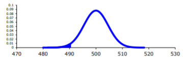.png?revision=1 "concept of hypothesis testing")
Before calculating the probability, it is useful to see how many standard deviations away from the mean the sample mean is. Using the formula for the z-score from chapter 6, you find
\(z=\dfrac{\overline{x}-\mu_{o}}{\sigma / \sqrt{n}}=\dfrac{490-500}{25 / \sqrt{30}}=-2.19\)
This sample mean is more than two standard deviations away from the mean. That seems pretty far, but you should look at the probability too.
On TI-83/84:
\(P(\overline{x}<490 | \mu=500)=\text { normalcdf }(-1 E 99,490,500,25 \div \sqrt{30}) \approx 0.0142\)
\(P(\overline{x}<490 \mu=500)=\text { pnorm }(490,500,25 / \operatorname{sqrt}(30)) \approx 0.0142\)
There is a 1.42% chance that you could find a sample mean less than 490 when the population mean is 500 days. This is really small, so the chances are that the assumption that the population mean is 500 days is wrong, and you can reject the manufacturer’s claim. But how do you quantify really small? Is 5% or 10% or 15% really small? How do you decide?
Before you answer that question, a couple more definitions are needed.
Definition \(\PageIndex{3}\)
Test Statistic : \(z=\dfrac{\overline{x}-\mu_{o}}{\sigma / \sqrt{n}}\) since it is calculated as part of the testing of the hypothesis.
Definition \(\PageIndex{4}\)
p – value : probability that the test statistic will take on more extreme values than the observed test statistic, given that the null hypothesis is true. It is the probability that was calculated above.
Now, how small is small enough? To answer that, you really want to know the types of errors you can make.
There are actually only two errors that can be made. The first error is if you say that \(H_{o}\) is false, when in fact it is true. This means you reject \(H_{o}\) when \(H_{o}\) was true. The second error is if you say that \(H_{o}\) is true, when in fact it is false. This means you fail to reject \(H_{o}\) when \(H_{o}\) is false. The following table organizes this for you:
Type of errors:
Definition \(\PageIndex{5}\)
Type I Error is rejecting \(H_{o}\) when \(H_{o}\) is true, and
Definition \(\PageIndex{6}\)
Type II Error is failing to reject \(H_{o}\) when \(H_{o}\) is false.
Since these are the errors, then one can define the probabilities attached to each error.
Definition \(\PageIndex{7}\)
\(\alpha\) = P(type I error) = P(rejecting \(H_{o} / H_{o}\) is true)
Definition \(\PageIndex{8}\)
\(\beta\) = P(type II error) = P(failing to reject \(H_{o} / H_{o}\) is false)
\(\alpha\) is also called the level of significance .
Another common concept that is used is Power = \(1-\beta \).
Now there is a relationship between \(\alpha\) and \(\beta\). They are not complements of each other. How are they related?
If \(\alpha\) increases that means the chances of making a type I error will increase. It is more likely that a type I error will occur. It makes sense that you are less likely to make type II errors, only because you will be rejecting \(H_{o}\) more often. You will be failing to reject \(H_{o}\) less, and therefore, the chance of making a type II error will decrease. Thus, as \(\alpha\) increases, \(\beta\) will decrease, and vice versa. That makes them seem like complements, but they aren’t complements. What gives? Consider one more factor – sample size.
Consider if you have a larger sample that is representative of the population, then it makes sense that you have more accuracy then with a smaller sample. Think of it this way, which would you trust more, a sample mean of 490 if you had a sample size of 35 or sample size of 350 (assuming a representative sample)? Of course the 350 because there are more data points and so more accuracy. If you are more accurate, then there is less chance that you will make any error. By increasing the sample size of a representative sample, you decrease both \(\alpha\) and \(\beta\).
Summary of all of this:
- For a certain sample size, n , if \(\alpha\) increases, \(\beta\) decreases.
- For a certain level of significance, \(\alpha\), if n increases, \(\beta\) decreases.
Now how do you find \(\alpha\) and \(\beta\)? Well \(\alpha\) is actually chosen. There are only three values that are usually picked for \(\alpha\): 0.01, 0.05, and 0.10. \(\beta\) is very difficult to find, so usually it isn’t found. If you want to make sure it is small you take as large of a sample as you can afford provided it is a representative sample. This is one use of the Power. You want \(\beta\) to be small and the Power of the test is large. The Power word sounds good.
Which pick of \(\alpha\) do you pick? Well that depends on what you are working on. Remember in this example you are the buyer who is trying to get out of a contract to buy these batteries. If you create a type I error, you said that the batteries are bad when they aren’t, most likely the manufacturer will sue you. You want to avoid this. You might pick \(\alpha\) to be 0.01. This way you have a small chance of making a type I error. Of course this means you have more of a chance of making a type II error. No big deal right? What if the batteries are used in pacemakers and you tell the person that their pacemaker’s batteries are good for 500 days when they actually last less, that might be bad. If you make a type II error, you say that the batteries do last 500 days when they last less, then you have the possibility of killing someone. You certainly do not want to do this. In this case you might want to pick \(\alpha\) as 0.10. If both errors are equally bad, then pick \(\alpha\) as 0.05.
The above discussion is why the choice of \(\alpha\) depends on what you are researching. As the researcher, you are the one that needs to decide what \(\alpha\) level to use based on your analysis of the consequences of making each error is.
If a type I error is really bad, then pick \(\alpha\) = 0.01.
If a type II error is really bad, then pick \(\alpha\) = 0.10
If neither error is bad, or both are equally bad, then pick \(\alpha\) = 0.05
The main thing is to always pick the \(\alpha\) before you collect the data and start the test.
The above discussion was long, but it is really important information. If you don’t know what the errors of the test are about, then there really is no point in making conclusions with the tests. Make sure you understand what the two errors are and what the probabilities are for them.
Now it is time to go back to the example and put this all together. This is the basic structure of testing a hypothesis, usually called a hypothesis test. Since this one has a test statistic involving z, it is also called a z-test. And since there is only one sample, it is usually called a one-sample z-test.
Example \(\PageIndex{2}\) battery example revisited
- State the random variable and the parameter in words.
- State the null and alternative hypothesis and the level of significance.
- A random sample of size n is taken.
- The population standard derivation is known.
- The sample size is at least 30 or the population of the random variable is normally distributed.
- Find the sample statistic, test statistic, and p-value.
- Interpretation
1. x = life of battery
\(\mu\) = mean life of a XJ35 battery
2. \(H_{o} : \mu=500\) days
\(H_{A} : \mu<500\) days
\(\alpha = 0.10\) (from above discussion about consequences)
3. Every hypothesis has some assumptions that be met to make sure that the results of the hypothesis are valid. The assumptions are different for each test. This test has the following assumptions.
- This occurred in this example, since it was stated that a random sample of 30 battery lives were taken.
- This is true, since it was given in the problem.
- The sample size was 30, so this condition is met.
4. The test statistic depends on how many samples there are, what parameter you are testing, and assumptions that need to be checked. In this case, there is one sample and you are testing the mean. The assumptions were checked above.
Sample statistic:
\(\overline{x} = 490\)
Test statistic:
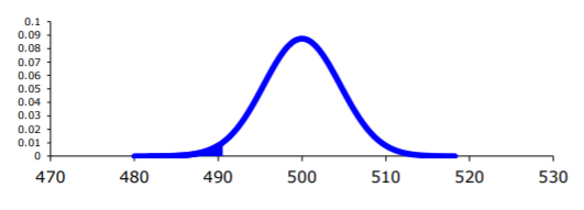.png?revision=1 "concept of hypothesis testing")
Using TI-83/84:
\(P(\overline{x}<490 | \mu=500)=\text { normalcdf }(-1 \mathrm{E} 99,490,500,25 / \sqrt{30}) \approx 0.0142\)
\(P(\overline{x}<490 | \mu=500)=\operatorname{pnorm}(490,500,25 / \operatorname{sqrt}(30)) \approx 0.0142\)
5. Now what? Well, this p-value is 0.0142. This is a lot smaller than the amount of error you would accept in the problem -\(\alpha\) = 0.10. That means that finding a sample mean less than 490 days is unusual to happen if \(H_{o}\) is true. This should make you think that \(H_{o}\) is not true. You should reject \(H_{o}\).
In fact, in general:
Reject \(H_{o}\) if the p-value < \(\alpha\) and
Fail to reject \(H_{o}\) if the p-value \(\geq \alpha\).
6. Since you rejected \(H_{o}\), what does this mean in the real world? That is what goes in the interpretation. Since you rejected the claim by the manufacturer that the mean life of the batteries is 500 days, then you now can believe that your hypothesis was correct. In other words, there is enough evidence to show that the mean life of the battery is less than 500 days.
Now that you know that the batteries last less than 500 days, should you cancel the contract? Statistically, there is evidence that the batteries do not last as long as the manufacturer says they should. However, based on this sample there are only ten days less on average that the batteries last. There may not be practical significance in this case. Ten days do not seem like a large difference. In reality, if the batteries are used in pacemakers, then you would probably tell the patient to have the batteries replaced every year. You have a large buffer whether the batteries last 490 days or 500 days. It seems that it might not be worth it to break the contract over ten days. What if the 10 days was practically significant? Are there any other things you should consider? You might look at the business relationship with the manufacturer. You might also look at how much it would cost to find a new manufacturer. These are also questions to consider before making any changes. What this discussion should show you is that just because a hypothesis has statistical significance does not mean it has practical significance. The hypothesis test is just one part of a research process. There are other pieces that you need to consider.
That’s it. That is what a hypothesis test looks like. All hypothesis tests are done with the same six steps. Those general six steps are outlined below.
- State the random variable and the parameter in words. This is where you are defining what the unknowns are in this problem. x = random variable \(\mu\) = mean of random variable, if the parameter of interest is the mean. There are other parameters you can test, and you would use the appropriate symbol for that parameter.
- State the null and alternative hypotheses and the level of significance \(H_{o} : \mu=\mu_{o}\), where \(\mu_{o}\) is the known mean \(H_{A} : \mu<\mu_{o}\) \(H_{A} : \mu>\mu_{o}\), use the appropriate one for your problem \(H_{A} : \mu \neq \mu_{o}\) Also, state your \(\alpha\) level here.
- State and check the assumptions for a hypothesis test. Each hypothesis test has its own assumptions. They will be stated when the different hypothesis tests are discussed.
- Find the sample statistic, test statistic, and p-value. This depends on what parameter you are working with, how many samples, and the assumptions of the test. The p-value depends on your \(H_{A}\). If you are doing the \(H_{A}\) with the less than, then it is a left-tailed test, and you find the probability of being in that left tail. If you are doing the \(H_{A}\) with the greater than, then it is a right-tailed test, and you find the probability of being in the right tail. If you are doing the \(H_{A}\) with the not equal to, then you are doing a two-tail test, and you find the probability of being in both tails. Because of symmetry, you could find the probability in one tail and double this value to find the probability in both tails.
- Conclusion This is where you write reject \(H_{o}\) or fail to reject \(H_{o}\). The rule is: if the p-value < \(\alpha\), then reject \(H_{o}\). If the p-value \(\geq \alpha\), then fail to reject \(H_{o}\).
- Interpretation This is where you interpret in real world terms the conclusion to the test. The conclusion for a hypothesis test is that you either have enough evidence to show \(H_{A}\) is true, or you do not have enough evidence to show \(H_{A}\) is true.
Sorry, one more concept about the conclusion and interpretation. First, the conclusion is that you reject \(H_{o}\) or you fail to reject \(H_{o}\). Why was it said like this? It is because you never accept the null hypothesis. If you wanted to accept the null hypothesis, then why do the test in the first place? In the interpretation, you either have enough evidence to show \(H_{A}\) is true, or you do not have enough evidence to show \(H_{A}\) is true. You wouldn’t want to go to all this work and then find out you wanted to accept the claim. Why go through the trouble? You always want to show that the alternative hypothesis is true. Sometimes you can do that and sometimes you can’t. It doesn’t mean you proved the null hypothesis; it just means you can’t prove the alternative hypothesis. Here is an example to demonstrate this.
Example \(\PageIndex{3}\) conclusion in hypothesis tests
In the U.S. court system a jury trial could be set up as a hypothesis test. To really help you see how this works, let’s use OJ Simpson as an example. In the court system, a person is presumed innocent until he/she is proven guilty, and this is your null hypothesis. OJ Simpson was a football player in the 1970s. In 1994 his ex-wife and her friend were killed. OJ Simpson was accused of the crime, and in 1995 the case was tried. The prosecutors wanted to prove OJ was guilty of killing his wife and her friend, and that is the alternative hypothesis
\(H_{0}\): OJ is innocent of killing his wife and her friend
\(H_{A}\): OJ is guilty of killing his wife and her friend
In this case, a verdict of not guilty was given. That does not mean that he is innocent of this crime. It means there was not enough evidence to prove he was guilty. Many people believe that OJ was guilty of this crime, but the jury did not feel that the evidence presented was enough to show there was guilt. The verdict in a jury trial is always guilty or not guilty!
The same is true in a hypothesis test. There is either enough or not enough evidence to show that alternative hypothesis. It is not that you proved the null hypothesis true.
When identifying hypothesis, it is important to state your random variable and the appropriate parameter you want to make a decision about. If count something, then the random variable is the number of whatever you counted. The parameter is the proportion of what you counted. If the random variable is something you measured, then the parameter is the mean of what you measured. (Note: there are other parameters you can calculate, and some analysis of those will be presented in later chapters.)
Example \(\PageIndex{4}\) stating hypotheses
Identify the hypotheses necessary to test the following statements:
- The average salary of a teacher is more than $30,000.
- The proportion of students who like math is less than 10%.
- The average age of students in this class differs from 21.
a. x = salary of teacher
\(\mu\) = mean salary of teacher
The guess is that \(\mu>\$ 30,000\) and that is the alternative hypothesis.
The null hypothesis has the same parameter and number with an equal sign.
\(\begin{array}{l}{H_{0} : \mu=\$ 30,000} \\ {H_{A} : \mu>\$ 30,000}\end{array}\)
b. x = number od students who like math
p = proportion of students who like math
The guess is that p < 0.10 and that is the alternative hypothesis.
\(\begin{array}{l}{H_{0} : p=0.10} \\ {H_{A} : p<0.10}\end{array}\)
c. x = age of students in this class
\(\mu\) = mean age of students in this class
The guess is that \(\mu \neq 21\) and that is the alternative hypothesis.
\(\begin{array}{c}{H_{0} : \mu=21} \\ {H_{A} : \mu \neq 21}\end{array}\)
Example \(\PageIndex{5}\) Stating Type I and II Errors and Picking Level of Significance
- The plant-breeding department at a major university developed a new hybrid raspberry plant called YumYum Berry. Based on research data, the claim is made that from the time shoots are planted 90 days on average are required to obtain the first berry with a standard deviation of 9.2 days. A corporation that is interested in marketing the product tests 60 shoots by planting them and recording the number of days before each plant produces its first berry. The sample mean is 92.3 days. The corporation wants to know if the mean number of days is more than the 90 days claimed. State the type I and type II errors in terms of this problem, consequences of each error, and state which level of significance to use.
- A concern was raised in Australia that the percentage of deaths of Aboriginal prisoners was higher than the percent of deaths of non-indigenous prisoners, which is 0.27%. State the type I and type II errors in terms of this problem, consequences of each error, and state which level of significance to use.
a. x = time to first berry for YumYum Berry plant
\(\mu\) = mean time to first berry for YumYum Berry plant
\(\begin{array}{l}{H_{0} : \mu=90} \\ {H_{A} : \mu>90}\end{array}\)
Type I Error: If the corporation does a type I error, then they will say that the plants take longer to produce than 90 days when they don’t. They probably will not want to market the plants if they think they will take longer. They will not market them even though in reality the plants do produce in 90 days. They may have loss of future earnings, but that is all.
Type II error: The corporation do not say that the plants take longer then 90 days to produce when they do take longer. Most likely they will market the plants. The plants will take longer, and so customers might get upset and then the company would get a bad reputation. This would be really bad for the company.
Level of significance: It appears that the corporation would not want to make a type II error. Pick a 10% level of significance, \(\alpha = 0.10\).
b. x = number of Aboriginal prisoners who have died
p = proportion of Aboriginal prisoners who have died
\(\begin{array}{l}{H_{o} : p=0.27 \%} \\ {H_{A} : p>0.27 \%}\end{array}\)
Type I error: Rejecting that the proportion of Aboriginal prisoners who died was 0.27%, when in fact it was 0.27%. This would mean you would say there is a problem when there isn’t one. You could anger the Aboriginal community, and spend time and energy researching something that isn’t a problem.
Type II error: Failing to reject that the proportion of Aboriginal prisoners who died was 0.27%, when in fact it is higher than 0.27%. This would mean that you wouldn’t think there was a problem with Aboriginal prisoners dying when there really is a problem. You risk causing deaths when there could be a way to avoid them.
Level of significance: It appears that both errors may be issues in this case. You wouldn’t want to anger the Aboriginal community when there isn’t an issue, and you wouldn’t want people to die when there may be a way to stop it. It may be best to pick a 5% level of significance, \(\alpha = 0.05\).
Hypothesis testing is really easy if you follow the same recipe every time. The only differences in the various problems are the assumptions of the test and the test statistic you calculate so you can find the p-value. Do the same steps, in the same order, with the same words, every time and these problems become very easy.
Exercise \(\PageIndex{1}\)
For the problems in this section, a question is being asked. This is to help you understand what the hypotheses are. You are not to run any hypothesis tests and come up with any conclusions in this section.
- Eyeglassomatic manufactures eyeglasses for different retailers. They test to see how many defective lenses they made in a given time period and found that 11% of all lenses had defects of some type. Looking at the type of defects, they found in a three-month time period that out of 34,641 defective lenses, 5865 were due to scratches. Are there more defects from scratches than from all other causes? State the random variable, population parameter, and hypotheses.
- According to the February 2008 Federal Trade Commission report on consumer fraud and identity theft, 23% of all complaints in 2007 were for identity theft. In that year, Alaska had 321 complaints of identity theft out of 1,432 consumer complaints ("Consumer fraud and," 2008). Does this data provide enough evidence to show that Alaska had a lower proportion of identity theft than 23%? State the random variable, population parameter, and hypotheses.
- The Kyoto Protocol was signed in 1997, and required countries to start reducing their carbon emissions. The protocol became enforceable in February 2005. In 2004, the mean CO2 emission was 4.87 metric tons per capita. Is there enough evidence to show that the mean CO2 emission is lower in 2010 than in 2004? State the random variable, population parameter, and hypotheses.
- The FDA regulates that fish that is consumed is allowed to contain 1.0 mg/kg of mercury. In Florida, bass fish were collected in 53 different lakes to measure the amount of mercury in the fish. The data for the average amount of mercury in each lake is in Example \(\PageIndex{5}\) ("Multi-disciplinary niser activity," 2013). Do the data provide enough evidence to show that the fish in Florida lakes has more mercury than the allowable amount? State the random variable, population parameter, and hypotheses.
- Eyeglassomatic manufactures eyeglasses for different retailers. They test to see how many defective lenses they made in a given time period and found that 11% of all lenses had defects of some type. Looking at the type of defects, they found in a three-month time period that out of 34,641 defective lenses, 5865 were due to scratches. Are there more defects from scratches than from all other causes? State the type I and type II errors in this case, consequences of each error type for this situation from the perspective of the manufacturer, and the appropriate alpha level to use. State why you picked this alpha level.
- According to the February 2008 Federal Trade Commission report on consumer fraud and identity theft, 23% of all complaints in 2007 were for identity theft. In that year, Alaska had 321 complaints of identity theft out of 1,432 consumer complaints ("Consumer fraud and," 2008). Does this data provide enough evidence to show that Alaska had a lower proportion of identity theft than 23%? State the type I and type II errors in this case, consequences of each error type for this situation from the perspective of the state of Arizona, and the appropriate alpha level to use. State why you picked this alpha level.
- The Kyoto Protocol was signed in 1997, and required countries to start reducing their carbon emissions. The protocol became enforceable in February 2005. In 2004, the mean CO2 emission was 4.87 metric tons per capita. Is there enough evidence to show that the mean CO2 emission is lower in 2010 than in 2004? State the type I and type II errors in this case, consequences of each error type for this situation from the perspective of the agency overseeing the protocol, and the appropriate alpha level to use. State why you picked this alpha level.
- The FDA regulates that fish that is consumed is allowed to contain 1.0 mg/kg of mercury. In Florida, bass fish were collected in 53 different lakes to measure the amount of mercury in the fish. The data for the average amount of mercury in each lake is in Example \(\PageIndex{5}\) ("Multi-disciplinary niser activity," 2013). Do the data provide enough evidence to show that the fish in Florida lakes has more mercury than the allowable amount? State the type I and type II errors in this case, consequences of each error type for this situation from the perspective of the FDA, and the appropriate alpha level to use. State why you picked this alpha level.
1. \(H_{o} : p=0.11, H_{A} : p>0.11\)
3. \(H_{o} : \mu=4.87 \text { metric tons per capita, } H_{A} : \mu<4.87 \text { metric tons per capita }\)
5. See solutions
7. See solutions
Module 8: Inference for One Proportion
Hypothesis testing (1 of 5), learning outcomes.
- When testing a claim, distinguish among situations involving one population mean, one population proportion, two population means, or two population proportions.
- Given a claim about a population, determine null and alternative hypotheses.
Introduction
In inference, we use a sample to draw a conclusion about a population. Two types of inference are the focus of our work in this course:
- Estimate a population parameter with a confidence interval.
- Test a claim about a population parameter with a hypothesis test.
We can also use samples from two populations to compare those populations. In this situation, the two types of inference focus on differences in the parameters.
- Estimate a difference in population parameters with a confidence interval.
- Test a claim about a difference in population parameters with a hypothesis test.
In “Estimating a Population Proportion,” we learned to estimate a population proportion using a confidence interval. For example, we estimated the proportion of all Tallahassee Community College students who are female and the proportion of all American adults who used the Internet to obtain medical information in the previous month. We will revisit confidence intervals in future modules.
Now we look more carefully at how to test a claim with a hypothesis test. Statistical investigations begin with research questions. We begin our discussion of hypothesis tests with research questions that require us to test a claim. Later we look at how a claim becomes a hypothesis.
Research Questions about Testing Claims

Let’s revisit some of the research questions from examples in the module Types of Statistical Studies and Producing Data that involve testing a claim.
Is the average course load for community college students less than 12 semester hours? This question contains a claim about a population mean. The question contains information about the population, the variable, and the parameter. The population is all community college students. The variable is course load in semester hours . It is quantitative, so the parameter is a mean. The claim is, “The mean course load for all community college students is less than 12 semester hours.”
Do the majority of community college students qualify for federal student loans? This question contains a claim about a population proportion and information about the population, the variable, and the parameter. The population is all community college students. The variable is Qualify for federal student loan (yes or no). It is categorical, so the parameter is a proportion. The claim is, “The proportion of community college students who qualify is greater than 0.5” (a majority means more than half, or 0.5).
In community colleges, do female students and male students have different mean GPAs? This question contains a claim that compares two population means. Again, we see information about the populations, the variable, and the parameters. The two populations are female community college students and male community college students. The variable is GPA . It is quantitative, so the parameters are means. The claim is, “The mean GPA for female community college students is different from the mean GPA for male community college students.” Notice that the claim compares the two population means, but there is no claim about the numeric value of either mean.
Are college athletes more likely than nonathletes to receive academic advising? This question contains a claim that compares two population proportions: college athletes and college students who are not athletes. The variable is Receive academic advising (yes or no). The variable is categorical, so the parameters are proportions. The claim is, “The proportion of all college athletes who receive academic advising is greater than the proportion of all nonathletes in college who receive academic advising.” Notice that the claim compares two population proportions, but there is no claim about the numeric value of either proportion.
In the case of testing a claim about a single population parameter, we compare it to a numeric value. In the case of testing a claim about two population parameters, we compare them to each other.
Identify the type of claim in each research question below.
Next Steps: Forming Hypotheses
We already know that in inference we use a sample to draw a conclusion about a population. If the research question contains a claim about the population, we translate the claim into two related hypotheses.
The null hypothesis is a hypothesis about the value of the parameter. The null hypothesis relates to our work in Linking Probability to Statistical Inference where we drew a conclusion about a population parameter on the basis of the sampling distribution. We started with an assumption about the value of the parameter, then used a simulation to simulate the selection of random samples from a population with this parameter value. Or we used the parameter value in a mathematical model to describe the center and spread of the sampling distribution. The null hypothesis gives the value of the parameter that we will use to create the sampling distribution. In this way, the null hypothesis states what we assume to be true about the population.
The alternative hypothesis usually reflects the claim in the research question about the value of the parameter. The alternative hypothesis says the parameter is “greater than” or “less than” or “not equal to” the value we assume to true in the null hypothesis.
Stating Hypotheses
Here are the hypotheses for the research questions from the previous example. The null hypothesis is abbreviated H 0 . The alternative hypothesis is abbreviated H a .
Is the average course load for community college students less than 12 semester hours?
- H 0 : The mean course load for community college students is equal to 12 semester hours.
- H a : The mean course load for community college students is less than 12 semester hours.
Do the majority of community college students qualify for federal student loans?
- H 0 : The proportion of community college students who qualify for federal student loans is 0.5.
- H a : The proportion of community college students who qualify for federal student loans is greater than 0.5.
When the research question contains a claim that compares two populations, the null hypothesis states that the parameters are equal. We will see in Modules 9 and 10 that we translate the null hypothesis into a statement about “no difference” in parameter values. We revisit this idea in more depth later.
In community colleges, do female students and male students have different mean GPAs?
- H 0 : In community colleges, female and male students have the same mean GPAs.
- H a : In community colleges, female and male students have different mean GPAs.
Are college athletes more likely than nonathletes to receive academic advising?
- H 0 : In colleges, the proportion of athletes who receive academic advising is equal to the proportion of nonathletes who receive academic advising.
- H a : In colleges, the proportion of athletes who receive academic advising is greater than the proportion of nonathletes who receive academic advising.
Here are some general observations about null and alternative hypotheses.
- The hypotheses are competing claims about the parameter or about the comparison of parameters.
- Both hypotheses are statements about the same population parameter or same two population parameters.
- The null hypothesis contains an equal sign.
- The alternative hypothesis is always an inequality statement. It contains a “less than” or a “greater than” or a “not equal to” symbol.
- In a statistical investigation, we determine the research question, and thus the hypotheses, before we collect data.
The process of forming hypotheses, collecting data, and using the data to draw a conclusion about the hypotheses is called hypothesis testing .
Contribute!
Improve this page Learn More
- Concepts in Statistics. Provided by : Open Learning Initiative. Located at : http://oli.cmu.edu . License : CC BY: Attribution

Tutorial Playlist
Statistics tutorial, everything you need to know about the probability density function in statistics, the best guide to understand central limit theorem, an in-depth guide to measures of central tendency : mean, median and mode, the ultimate guide to understand conditional probability.
A Comprehensive Look at Percentile in Statistics
The Best Guide to Understand Bayes Theorem
Everything you need to know about the normal distribution, an in-depth explanation of cumulative distribution function, a complete guide to chi-square test, a complete guide on hypothesis testing in statistics, understanding the fundamentals of arithmetic and geometric progression, the definitive guide to understand spearman’s rank correlation, a comprehensive guide to understand mean squared error, all you need to know about the empirical rule in statistics, the complete guide to skewness and kurtosis, a holistic look at bernoulli distribution.
All You Need to Know About Bias in Statistics
A Complete Guide to Get a Grasp of Time Series Analysis
The Key Differences Between Z-Test Vs. T-Test
The Complete Guide to Understand Pearson's Correlation
A complete guide on the types of statistical studies, everything you need to know about poisson distribution, your best guide to understand correlation vs. regression, the most comprehensive guide for beginners on what is correlation, what is hypothesis testing in statistics types and examples.
Lesson 10 of 24 By Avijeet Biswal

Table of Contents
In today’s data-driven world , decisions are based on data all the time. Hypothesis plays a crucial role in that process, whether it may be making business decisions, in the health sector, academia, or in quality improvement. Without hypothesis & hypothesis tests, you risk drawing the wrong conclusions and making bad decisions. In this tutorial, you will look at Hypothesis Testing in Statistics.
What Is Hypothesis Testing in Statistics?
Hypothesis Testing is a type of statistical analysis in which you put your assumptions about a population parameter to the test. It is used to estimate the relationship between 2 statistical variables.
Let's discuss few examples of statistical hypothesis from real-life -
- A teacher assumes that 60% of his college's students come from lower-middle-class families.
- A doctor believes that 3D (Diet, Dose, and Discipline) is 90% effective for diabetic patients.
Now that you know about hypothesis testing, look at the two types of hypothesis testing in statistics.
Hypothesis Testing Formula
Z = ( x̅ – μ0 ) / (σ /√n)
- Here, x̅ is the sample mean,
- μ0 is the population mean,
- σ is the standard deviation,
- n is the sample size.
How Hypothesis Testing Works?
An analyst performs hypothesis testing on a statistical sample to present evidence of the plausibility of the null hypothesis. Measurements and analyses are conducted on a random sample of the population to test a theory. Analysts use a random population sample to test two hypotheses: the null and alternative hypotheses.
The null hypothesis is typically an equality hypothesis between population parameters; for example, a null hypothesis may claim that the population means return equals zero. The alternate hypothesis is essentially the inverse of the null hypothesis (e.g., the population means the return is not equal to zero). As a result, they are mutually exclusive, and only one can be correct. One of the two possibilities, however, will always be correct.
Your Dream Career is Just Around The Corner!
Null Hypothesis and Alternate Hypothesis
The Null Hypothesis is the assumption that the event will not occur. A null hypothesis has no bearing on the study's outcome unless it is rejected.
H0 is the symbol for it, and it is pronounced H-naught.
The Alternate Hypothesis is the logical opposite of the null hypothesis. The acceptance of the alternative hypothesis follows the rejection of the null hypothesis. H1 is the symbol for it.
Let's understand this with an example.
A sanitizer manufacturer claims that its product kills 95 percent of germs on average.
To put this company's claim to the test, create a null and alternate hypothesis.
H0 (Null Hypothesis): Average = 95%.
Alternative Hypothesis (H1): The average is less than 95%.
Another straightforward example to understand this concept is determining whether or not a coin is fair and balanced. The null hypothesis states that the probability of a show of heads is equal to the likelihood of a show of tails. In contrast, the alternate theory states that the probability of a show of heads and tails would be very different.
Become a Data Scientist with Hands-on Training!
Hypothesis Testing Calculation With Examples
Let's consider a hypothesis test for the average height of women in the United States. Suppose our null hypothesis is that the average height is 5'4". We gather a sample of 100 women and determine that their average height is 5'5". The standard deviation of population is 2.
To calculate the z-score, we would use the following formula:
z = ( x̅ – μ0 ) / (σ /√n)
z = (5'5" - 5'4") / (2" / √100)
z = 0.5 / (0.045)
We will reject the null hypothesis as the z-score of 11.11 is very large and conclude that there is evidence to suggest that the average height of women in the US is greater than 5'4".
Steps of Hypothesis Testing
Step 1: specify your null and alternate hypotheses.
It is critical to rephrase your original research hypothesis (the prediction that you wish to study) as a null (Ho) and alternative (Ha) hypothesis so that you can test it quantitatively. Your first hypothesis, which predicts a link between variables, is generally your alternate hypothesis. The null hypothesis predicts no link between the variables of interest.
Step 2: Gather Data
For a statistical test to be legitimate, sampling and data collection must be done in a way that is meant to test your hypothesis. You cannot draw statistical conclusions about the population you are interested in if your data is not representative.
Step 3: Conduct a Statistical Test
Other statistical tests are available, but they all compare within-group variance (how to spread out the data inside a category) against between-group variance (how different the categories are from one another). If the between-group variation is big enough that there is little or no overlap between groups, your statistical test will display a low p-value to represent this. This suggests that the disparities between these groups are unlikely to have occurred by accident. Alternatively, if there is a large within-group variance and a low between-group variance, your statistical test will show a high p-value. Any difference you find across groups is most likely attributable to chance. The variety of variables and the level of measurement of your obtained data will influence your statistical test selection.
Step 4: Determine Rejection Of Your Null Hypothesis
Your statistical test results must determine whether your null hypothesis should be rejected or not. In most circumstances, you will base your judgment on the p-value provided by the statistical test. In most circumstances, your preset level of significance for rejecting the null hypothesis will be 0.05 - that is, when there is less than a 5% likelihood that these data would be seen if the null hypothesis were true. In other circumstances, researchers use a lower level of significance, such as 0.01 (1%). This reduces the possibility of wrongly rejecting the null hypothesis.
Step 5: Present Your Results
The findings of hypothesis testing will be discussed in the results and discussion portions of your research paper, dissertation, or thesis. You should include a concise overview of the data and a summary of the findings of your statistical test in the results section. You can talk about whether your results confirmed your initial hypothesis or not in the conversation. Rejecting or failing to reject the null hypothesis is a formal term used in hypothesis testing. This is likely a must for your statistics assignments.
Types of Hypothesis Testing
To determine whether a discovery or relationship is statistically significant, hypothesis testing uses a z-test. It usually checks to see if two means are the same (the null hypothesis). Only when the population standard deviation is known and the sample size is 30 data points or more, can a z-test be applied.
A statistical test called a t-test is employed to compare the means of two groups. To determine whether two groups differ or if a procedure or treatment affects the population of interest, it is frequently used in hypothesis testing.
Chi-Square
You utilize a Chi-square test for hypothesis testing concerning whether your data is as predicted. To determine if the expected and observed results are well-fitted, the Chi-square test analyzes the differences between categorical variables from a random sample. The test's fundamental premise is that the observed values in your data should be compared to the predicted values that would be present if the null hypothesis were true.
Hypothesis Testing and Confidence Intervals
Both confidence intervals and hypothesis tests are inferential techniques that depend on approximating the sample distribution. Data from a sample is used to estimate a population parameter using confidence intervals. Data from a sample is used in hypothesis testing to examine a given hypothesis. We must have a postulated parameter to conduct hypothesis testing.
Bootstrap distributions and randomization distributions are created using comparable simulation techniques. The observed sample statistic is the focal point of a bootstrap distribution, whereas the null hypothesis value is the focal point of a randomization distribution.
A variety of feasible population parameter estimates are included in confidence ranges. In this lesson, we created just two-tailed confidence intervals. There is a direct connection between these two-tail confidence intervals and these two-tail hypothesis tests. The results of a two-tailed hypothesis test and two-tailed confidence intervals typically provide the same results. In other words, a hypothesis test at the 0.05 level will virtually always fail to reject the null hypothesis if the 95% confidence interval contains the predicted value. A hypothesis test at the 0.05 level will nearly certainly reject the null hypothesis if the 95% confidence interval does not include the hypothesized parameter.
Simple and Composite Hypothesis Testing
Depending on the population distribution, you can classify the statistical hypothesis into two types.
Simple Hypothesis: A simple hypothesis specifies an exact value for the parameter.
Composite Hypothesis: A composite hypothesis specifies a range of values.
A company is claiming that their average sales for this quarter are 1000 units. This is an example of a simple hypothesis.
Suppose the company claims that the sales are in the range of 900 to 1000 units. Then this is a case of a composite hypothesis.
One-Tailed and Two-Tailed Hypothesis Testing
The One-Tailed test, also called a directional test, considers a critical region of data that would result in the null hypothesis being rejected if the test sample falls into it, inevitably meaning the acceptance of the alternate hypothesis.
In a one-tailed test, the critical distribution area is one-sided, meaning the test sample is either greater or lesser than a specific value.
In two tails, the test sample is checked to be greater or less than a range of values in a Two-Tailed test, implying that the critical distribution area is two-sided.
If the sample falls within this range, the alternate hypothesis will be accepted, and the null hypothesis will be rejected.
Become a Data Scientist With Real-World Experience
Right Tailed Hypothesis Testing
If the larger than (>) sign appears in your hypothesis statement, you are using a right-tailed test, also known as an upper test. Or, to put it another way, the disparity is to the right. For instance, you can contrast the battery life before and after a change in production. Your hypothesis statements can be the following if you want to know if the battery life is longer than the original (let's say 90 hours):
- The null hypothesis is (H0 <= 90) or less change.
- A possibility is that battery life has risen (H1) > 90.
The crucial point in this situation is that the alternate hypothesis (H1), not the null hypothesis, decides whether you get a right-tailed test.
Left Tailed Hypothesis Testing
Alternative hypotheses that assert the true value of a parameter is lower than the null hypothesis are tested with a left-tailed test; they are indicated by the asterisk "<".
Suppose H0: mean = 50 and H1: mean not equal to 50
According to the H1, the mean can be greater than or less than 50. This is an example of a Two-tailed test.
In a similar manner, if H0: mean >=50, then H1: mean <50
Here the mean is less than 50. It is called a One-tailed test.
Type 1 and Type 2 Error
A hypothesis test can result in two types of errors.
Type 1 Error: A Type-I error occurs when sample results reject the null hypothesis despite being true.
Type 2 Error: A Type-II error occurs when the null hypothesis is not rejected when it is false, unlike a Type-I error.
Suppose a teacher evaluates the examination paper to decide whether a student passes or fails.
H0: Student has passed
H1: Student has failed
Type I error will be the teacher failing the student [rejects H0] although the student scored the passing marks [H0 was true].
Type II error will be the case where the teacher passes the student [do not reject H0] although the student did not score the passing marks [H1 is true].
Level of Significance
The alpha value is a criterion for determining whether a test statistic is statistically significant. In a statistical test, Alpha represents an acceptable probability of a Type I error. Because alpha is a probability, it can be anywhere between 0 and 1. In practice, the most commonly used alpha values are 0.01, 0.05, and 0.1, which represent a 1%, 5%, and 10% chance of a Type I error, respectively (i.e. rejecting the null hypothesis when it is in fact correct).
Future-Proof Your AI/ML Career: Top Dos and Don'ts
A p-value is a metric that expresses the likelihood that an observed difference could have occurred by chance. As the p-value decreases the statistical significance of the observed difference increases. If the p-value is too low, you reject the null hypothesis.
Here you have taken an example in which you are trying to test whether the new advertising campaign has increased the product's sales. The p-value is the likelihood that the null hypothesis, which states that there is no change in the sales due to the new advertising campaign, is true. If the p-value is .30, then there is a 30% chance that there is no increase or decrease in the product's sales. If the p-value is 0.03, then there is a 3% probability that there is no increase or decrease in the sales value due to the new advertising campaign. As you can see, the lower the p-value, the chances of the alternate hypothesis being true increases, which means that the new advertising campaign causes an increase or decrease in sales.
Why is Hypothesis Testing Important in Research Methodology?
Hypothesis testing is crucial in research methodology for several reasons:
- Provides evidence-based conclusions: It allows researchers to make objective conclusions based on empirical data, providing evidence to support or refute their research hypotheses.
- Supports decision-making: It helps make informed decisions, such as accepting or rejecting a new treatment, implementing policy changes, or adopting new practices.
- Adds rigor and validity: It adds scientific rigor to research using statistical methods to analyze data, ensuring that conclusions are based on sound statistical evidence.
- Contributes to the advancement of knowledge: By testing hypotheses, researchers contribute to the growth of knowledge in their respective fields by confirming existing theories or discovering new patterns and relationships.
Limitations of Hypothesis Testing
Hypothesis testing has some limitations that researchers should be aware of:
- It cannot prove or establish the truth: Hypothesis testing provides evidence to support or reject a hypothesis, but it cannot confirm the absolute truth of the research question.
- Results are sample-specific: Hypothesis testing is based on analyzing a sample from a population, and the conclusions drawn are specific to that particular sample.
- Possible errors: During hypothesis testing, there is a chance of committing type I error (rejecting a true null hypothesis) or type II error (failing to reject a false null hypothesis).
- Assumptions and requirements: Different tests have specific assumptions and requirements that must be met to accurately interpret results.
After reading this tutorial, you would have a much better understanding of hypothesis testing, one of the most important concepts in the field of Data Science . The majority of hypotheses are based on speculation about observed behavior, natural phenomena, or established theories.
If you are interested in statistics of data science and skills needed for such a career, you ought to explore Simplilearn’s Post Graduate Program in Data Science.
If you have any questions regarding this ‘Hypothesis Testing In Statistics’ tutorial, do share them in the comment section. Our subject matter expert will respond to your queries. Happy learning!
1. What is hypothesis testing in statistics with example?
Hypothesis testing is a statistical method used to determine if there is enough evidence in a sample data to draw conclusions about a population. It involves formulating two competing hypotheses, the null hypothesis (H0) and the alternative hypothesis (Ha), and then collecting data to assess the evidence. An example: testing if a new drug improves patient recovery (Ha) compared to the standard treatment (H0) based on collected patient data.
2. What is hypothesis testing and its types?
Hypothesis testing is a statistical method used to make inferences about a population based on sample data. It involves formulating two hypotheses: the null hypothesis (H0), which represents the default assumption, and the alternative hypothesis (Ha), which contradicts H0. The goal is to assess the evidence and determine whether there is enough statistical significance to reject the null hypothesis in favor of the alternative hypothesis.
Types of hypothesis testing:
- One-sample test: Used to compare a sample to a known value or a hypothesized value.
- Two-sample test: Compares two independent samples to assess if there is a significant difference between their means or distributions.
- Paired-sample test: Compares two related samples, such as pre-test and post-test data, to evaluate changes within the same subjects over time or under different conditions.
- Chi-square test: Used to analyze categorical data and determine if there is a significant association between variables.
- ANOVA (Analysis of Variance): Compares means across multiple groups to check if there is a significant difference between them.
3. What are the steps of hypothesis testing?
The steps of hypothesis testing are as follows:
- Formulate the hypotheses: State the null hypothesis (H0) and the alternative hypothesis (Ha) based on the research question.
- Set the significance level: Determine the acceptable level of error (alpha) for making a decision.
- Collect and analyze data: Gather and process the sample data.
- Compute test statistic: Calculate the appropriate statistical test to assess the evidence.
- Make a decision: Compare the test statistic with critical values or p-values and determine whether to reject H0 in favor of Ha or not.
- Draw conclusions: Interpret the results and communicate the findings in the context of the research question.
4. What are the 2 types of hypothesis testing?
- One-tailed (or one-sided) test: Tests for the significance of an effect in only one direction, either positive or negative.
- Two-tailed (or two-sided) test: Tests for the significance of an effect in both directions, allowing for the possibility of a positive or negative effect.
The choice between one-tailed and two-tailed tests depends on the specific research question and the directionality of the expected effect.
5. What are the 3 major types of hypothesis?
The three major types of hypotheses are:
- Null Hypothesis (H0): Represents the default assumption, stating that there is no significant effect or relationship in the data.
- Alternative Hypothesis (Ha): Contradicts the null hypothesis and proposes a specific effect or relationship that researchers want to investigate.
- Nondirectional Hypothesis: An alternative hypothesis that doesn't specify the direction of the effect, leaving it open for both positive and negative possibilities.
Find our Data Analyst Online Bootcamp in top cities:
About the author.
Avijeet is a Senior Research Analyst at Simplilearn. Passionate about Data Analytics, Machine Learning, and Deep Learning, Avijeet is also interested in politics, cricket, and football.
Recommended Resources
Free eBook: Top Programming Languages For A Data Scientist
Normality Test in Minitab: Minitab with Statistics
Machine Learning Career Guide: A Playbook to Becoming a Machine Learning Engineer
- PMP, PMI, PMBOK, CAPM, PgMP, PfMP, ACP, PBA, RMP, SP, and OPM3 are registered marks of the Project Management Institute, Inc.

- school Campus Bookshelves
- menu_book Bookshelves
- perm_media Learning Objects
- login Login
- how_to_reg Request Instructor Account
- hub Instructor Commons
- Download Page (PDF)
- Download Full Book (PDF)
- Periodic Table
- Physics Constants
- Scientific Calculator
- Reference & Cite
- Tools expand_more
- Readability
selected template will load here
This action is not available.
8.1: The Elements of Hypothesis Testing
- Last updated
- Save as PDF
- Page ID 130263
Learning Objectives
- To understand the logical framework of tests of hypotheses.
- To learn basic terminology connected with hypothesis testing.
- To learn fundamental facts about hypothesis testing.
Types of Hypotheses
A hypothesis about the value of a population parameter is an assertion about its value. As in the introductory example we will be concerned with testing the truth of two competing hypotheses, only one of which can be true.
Definition: null hypothesis and alternative hypothesis
- The null hypothesis , denoted \(H_0\), is the statement about the population parameter that is assumed to be true unless there is convincing evidence to the contrary.
- The alternative hypothesis , denoted \(H_a\), is a statement about the population parameter that is contradictory to the null hypothesis, and is accepted as true only if there is convincing evidence in favor of it.
Definition: statistical procedure
Hypothesis testing is a statistical procedure in which a choice is made between a null hypothesis and an alternative hypothesis based on information in a sample.
The end result of a hypotheses testing procedure is a choice of one of the following two possible conclusions:
- Reject \(H_0\) (and therefore accept \(H_a\)), or
- Fail to reject \(H_0\) (and therefore fail to accept \(H_a\)).
The null hypothesis typically represents the status quo, or what has historically been true. In the example of the respirators, we would believe the claim of the manufacturer unless there is reason not to do so, so the null hypotheses is \(H_0:\mu =75\). The alternative hypothesis in the example is the contradictory statement \(H_a:\mu <75\). The null hypothesis will always be an assertion containing an equals sign, but depending on the situation the alternative hypothesis can have any one of three forms: with the symbol \(<\), as in the example just discussed, with the symbol \(>\), or with the symbol \(\neq\). The following two examples illustrate the latter two cases.
Example \(\PageIndex{1}\)
A publisher of college textbooks claims that the average price of all hardbound college textbooks is \(\$127.50\). A student group believes that the actual mean is higher and wishes to test their belief. State the relevant null and alternative hypotheses.
The default option is to accept the publisher’s claim unless there is compelling evidence to the contrary. Thus the null hypothesis is \(H_0:\mu =127.50\). Since the student group thinks that the average textbook price is greater than the publisher’s figure, the alternative hypothesis in this situation is \(H_a:\mu >127.50\).
Example \(\PageIndex{2}\)
The recipe for a bakery item is designed to result in a product that contains \(8\) grams of fat per serving. The quality control department samples the product periodically to insure that the production process is working as designed. State the relevant null and alternative hypotheses.
The default option is to assume that the product contains the amount of fat it was formulated to contain unless there is compelling evidence to the contrary. Thus the null hypothesis is \(H_0:\mu =8.0\). Since to contain either more fat than desired or to contain less fat than desired are both an indication of a faulty production process, the alternative hypothesis in this situation is that the mean is different from \(8.0\), so \(H_a:\mu \neq 8.0\).
In Example \(\PageIndex{1}\), the textbook example, it might seem more natural that the publisher’s claim be that the average price is at most \(\$127.50\), not exactly \(\$127.50\). If the claim were made this way, then the null hypothesis would be \(H_0:\mu \leq 127.50\), and the value \(\$127.50\) given in the example would be the one that is least favorable to the publisher’s claim, the null hypothesis. It is always true that if the null hypothesis is retained for its least favorable value, then it is retained for every other value.
Thus in order to make the null and alternative hypotheses easy for the student to distinguish, in every example and problem in this text we will always present one of the two competing claims about the value of a parameter with an equality. The claim expressed with an equality is the null hypothesis. This is the same as always stating the null hypothesis in the least favorable light. So in the introductory example about the respirators, we stated the manufacturer’s claim as “the average is \(75\) minutes” instead of the perhaps more natural “the average is at least \(75\) minutes,” essentially reducing the presentation of the null hypothesis to its worst case.
The first step in hypothesis testing is to identify the null and alternative hypotheses.
The Logic of Hypothesis Testing
Although we will study hypothesis testing in situations other than for a single population mean (for example, for a population proportion instead of a mean or in comparing the means of two different populations), in this section the discussion will always be given in terms of a single population mean \(\mu\).
The null hypothesis always has the form \(H_0:\mu =\mu _0\) for a specific number \(\mu _0\) (in the respirator example \(\mu _0=75\), in the textbook example \(\mu _0=127.50\), and in the baked goods example \(\mu _0=8.0\)). Since the null hypothesis is accepted unless there is strong evidence to the contrary, the test procedure is based on the initial assumption that \(H_0\) is true. This point is so important that we will repeat it in a display:
The test procedure is based on the initial assumption that \(H_0\) is true.
The criterion for judging between \(H_0\) and \(H_a\) based on the sample data is: if the value of \(\overline{X}\) would be highly unlikely to occur if \(H_0\) were true, but favors the truth of \(H_a\), then we reject \(H_0\) in favor of \(H_a\). Otherwise we do not reject \(H_0\).
Supposing for now that \(\overline{X}\) follows a normal distribution, when the null hypothesis is true the density function for the sample mean \(\overline{X}\) must be as in Figure \(\PageIndex{1}\): a bell curve centered at \(\mu _0\). Thus if \(H_0\) is true then \(\overline{X}\) is likely to take a value near \(\mu _0\) and is unlikely to take values far away. Our decision procedure therefore reduces simply to:
- if \(H_a\) has the form \(H_a:\mu <\mu _0\) then reject \(H_0\) if \(\bar{x}\) is far to the left of \(\mu _0\);
- if \(H_a\) has the form \(H_a:\mu >\mu _0\) then reject \(H_0\) if \(\bar{x}\) is far to the right of \(\mu _0\);
- if \(H_a\) has the form \(H_a:\mu \neq \mu _0\) then reject \(H_0\) if \(\bar{x}\) is far away from \(\mu _0\) in either direction.

Think of the respirator example, for which the null hypothesis is \(H_0:\mu =75\), the claim that the average time air is delivered for all respirators is \(75\) minutes. If the sample mean is \(75\) or greater then we certainly would not reject \(H_0\) (since there is no issue with an emergency respirator delivering air even longer than claimed).
If the sample mean is slightly less than \(75\) then we would logically attribute the difference to sampling error and also not reject \(H_0\) either.
Values of the sample mean that are smaller and smaller are less and less likely to come from a population for which the population mean is \(75\). Thus if the sample mean is far less than \(75\), say around \(60\) minutes or less, then we would certainly reject \(H_0\), because we know that it is highly unlikely that the average of a sample would be so low if the population mean were \(75\). This is the rare event criterion for rejection: what we actually observed \((\overline{X}<60)\) would be so rare an event if \(\mu =75\) were true that we regard it as much more likely that the alternative hypothesis \(\mu <75\) holds.
In summary, to decide between \(H_0\) and \(H_a\) in this example we would select a “rejection region” of values sufficiently far to the left of \(75\), based on the rare event criterion, and reject \(H_0\) if the sample mean \(\overline{X}\) lies in the rejection region, but not reject \(H_0\) if it does not.
The Rejection Region
Each different form of the alternative hypothesis Ha has its own kind of rejection region:
- if (as in the respirator example) \(H_a\) has the form \(H_a:\mu <\mu _0\), we reject \(H_0\) if \(\bar{x}\) is far to the left of \(\mu _0\), that is, to the left of some number \(C\), so the rejection region has the form of an interval \((-\infty ,C]\);
- if (as in the textbook example) \(H_a\) has the form \(H_a:\mu >\mu _0\), we reject \(H_0\) if \(\bar{x}\) is far to the right of \(\mu _0\), that is, to the right of some number \(C\), so the rejection region has the form of an interval \([C,\infty )\);
- if (as in the baked good example) \(H_a\) has the form \(H_a:\mu \neq \mu _0\), we reject \(H_0\) if \(\bar{x}\) is far away from \(\mu _0\) in either direction, that is, either to the left of some number \(C\) or to the right of some other number \(C′\), so the rejection region has the form of the union of two intervals \((-\infty ,C]\cup [C',\infty )\).
The key issue in our line of reasoning is the question of how to determine the number \(C\) or numbers \(C\) and \(C′\), called the critical value or critical values of the statistic, that determine the rejection region.
Definition: critical values
The critical value or critical values of a test of hypotheses are the number or numbers that determine the rejection region.
Suppose the rejection region is a single interval, so we need to select a single number \(C\). Here is the procedure for doing so. We select a small probability, denoted \(\alpha\), say \(1\%\), which we take as our definition of “rare event:” an event is “rare” if its probability of occurrence is less than \(\alpha\). (In all the examples and problems in this text the value of \(\alpha\) will be given already.) The probability that \(\overline{X}\) takes a value in an interval is the area under its density curve and above that interval, so as shown in Figure \(\PageIndex{2}\) (drawn under the assumption that \(H_0\) is true, so that the curve centers at \(\mu _0\)) the critical value \(C\) is the value of \(\overline{X}\) that cuts off a tail area \(\alpha\) in the probability density curve of \(\overline{X}\). When the rejection region is in two pieces, that is, composed of two intervals, the total area above both of them must be \(\alpha\), so the area above each one is \(\alpha /2\), as also shown in Figure \(\PageIndex{2}\).

The number \(\alpha\) is the total area of a tail or a pair of tails.
Example \(\PageIndex{3}\)
In the context of Example \(\PageIndex{2}\), suppose that it is known that the population is normally distributed with standard deviation \(\alpha =0.15\) gram, and suppose that the test of hypotheses \(H_0:\mu =8.0\) versus \(H_a:\mu \neq 8.0\) will be performed with a sample of size \(5\). Construct the rejection region for the test for the choice \(\alpha =0.10\). Explain the decision procedure and interpret it.
If \(H_0\) is true then the sample mean \(\overline{X}\) is normally distributed with mean and standard deviation
\[\begin{align} \mu _{\overline{X}} &=\mu \nonumber \\[5pt] &=8.0 \nonumber \end{align} \nonumber \]
\[\begin{align} \sigma _{\overline{X}}&=\dfrac{\sigma}{\sqrt{n}} \nonumber \\[5pt] &= \dfrac{0.15}{\sqrt{5}} \nonumber\\[5pt] &=0.067 \nonumber \end{align} \nonumber \]
Since \(H_a\) contains the \(\neq\) symbol the rejection region will be in two pieces, each one corresponding to a tail of area \(\alpha /2=0.10/2=0.05\). From Figure 7.1.6, \(z_{0.05}=1.645\), so \(C\) and \(C′\) are \(1.645\) standard deviations of \(\overline{X}\) to the right and left of its mean \(8.0\):
\[C=8.0-(1.645)(0.067) = 7.89 \; \; \text{and}\; \; C'=8.0 + (1.645)(0.067) = 8.11 \nonumber \]
The result is shown in Figure \(\PageIndex{3}\). α = 0.1

The decision procedure is: take a sample of size \(5\) and compute the sample mean \(\bar{x}\). If \(\bar{x}\) is either \(7.89\) grams or less or \(8.11\) grams or more then reject the hypothesis that the average amount of fat in all servings of the product is \(8.0\) grams in favor of the alternative that it is different from \(8.0\) grams. Otherwise do not reject the hypothesis that the average amount is \(8.0\) grams.
The reasoning is that if the true average amount of fat per serving were \(8.0\) grams then there would be less than a \(10\%\) chance that a sample of size \(5\) would produce a mean of either \(7.89\) grams or less or \(8.11\) grams or more. Hence if that happened it would be more likely that the value \(8.0\) is incorrect (always assuming that the population standard deviation is \(0.15\) gram).
Because the rejection regions are computed based on areas in tails of distributions, as shown in Figure \(\PageIndex{2}\), hypothesis tests are classified according to the form of the alternative hypothesis in the following way.
Definitions: Test classifications
- If \(H_a\) has the form \(\mu \neq \mu _0\) the test is called a two-tailed test .
- If \(H_a\) has the form \(\mu < \mu _0\) the test is called a left-tailed test .
- If \(H_a\) has the form \(\mu > \mu _0\)the test is called a right-tailed test .
Each of the last two forms is also called a one-tailed test .
Two Types of Errors
The format of the testing procedure in general terms is to take a sample and use the information it contains to come to a decision about the two hypotheses. As stated before our decision will always be either
- reject the null hypothesis \(H_0\) in favor of the alternative \(H_a\) presented, or
- do not reject the null hypothesis \(H_0\) in favor of the alternative \(H_0\) presented.
There are four possible outcomes of hypothesis testing procedure, as shown in the following table:
As the table shows, there are two ways to be right and two ways to be wrong. Typically to reject \(H_0\) when it is actually true is a more serious error than to fail to reject it when it is false, so the former error is labeled “ Type I ” and the latter error “ Type II ”.
Definition: Type I and Type II errors
In a test of hypotheses:
- A Type I error is the decision to reject \(H_0\) when it is in fact true.
- A Type II error is the decision not to reject \(H_0\) when it is in fact not true.
Unless we perform a census we do not have certain knowledge, so we do not know whether our decision matches the true state of nature or if we have made an error. We reject \(H_0\) if what we observe would be a “rare” event if \(H_0\) were true. But rare events are not impossible: they occur with probability \(\alpha\). Thus when \(H_0\) is true, a rare event will be observed in the proportion \(\alpha\) of repeated similar tests, and \(H_0\) will be erroneously rejected in those tests. Thus \(\alpha\) is the probability that in following the testing procedure to decide between \(H_0\) and \(H_a\) we will make a Type I error.
Definition: level of significance
The number \(\alpha\) that is used to determine the rejection region is called the level of significance of the test. It is the probability that the test procedure will result in a Type I error .
The probability of making a Type II error is too complicated to discuss in a beginning text, so we will say no more about it than this: for a fixed sample size, choosing \(alpha\) smaller in order to reduce the chance of making a Type I error has the effect of increasing the chance of making a Type II error . The only way to simultaneously reduce the chances of making either kind of error is to increase the sample size.
Standardizing the Test Statistic
Hypotheses testing will be considered in a number of contexts, and great unification as well as simplification results when the relevant sample statistic is standardized by subtracting its mean from it and then dividing by its standard deviation. The resulting statistic is called a standardized test statistic . In every situation treated in this and the following two chapters the standardized test statistic will have either the standard normal distribution or Student’s \(t\)-distribution.
Definition: hypothesis test
A standardized test statistic for a hypothesis test is the statistic that is formed by subtracting from the statistic of interest its mean and dividing by its standard deviation.
For example, reviewing Example \(\PageIndex{3}\), if instead of working with the sample mean \(\overline{X}\) we instead work with the test statistic
\[\frac{\overline{X}-8.0}{0.067} \nonumber \]
then the distribution involved is standard normal and the critical values are just \(\pm z_{0.05}\). The extra work that was done to find that \(C=7.89\) and \(C′=8.11\) is eliminated. In every hypothesis test in this book the standardized test statistic will be governed by either the standard normal distribution or Student’s \(t\)-distribution. Information about rejection regions is summarized in the following tables:
Every instance of hypothesis testing discussed in this and the following two chapters will have a rejection region like one of the six forms tabulated in the tables above.
No matter what the context a test of hypotheses can always be performed by applying the following systematic procedure, which will be illustrated in the examples in the succeeding sections.
Systematic Hypothesis Testing Procedure: Critical Value Approach
- Identify the null and alternative hypotheses.
- Identify the relevant test statistic and its distribution.
- Compute from the data the value of the test statistic.
- Construct the rejection region.
- Compare the value computed in Step 3 to the rejection region constructed in Step 4 and make a decision. Formulate the decision in the context of the problem, if applicable.
The procedure that we have outlined in this section is called the “Critical Value Approach” to hypothesis testing to distinguish it from an alternative but equivalent approach that will be introduced at the end of Section 8.3.
Key Takeaway
- A test of hypotheses is a statistical process for deciding between two competing assertions about a population parameter.
- The testing procedure is formalized in a five-step procedure.
Talk to our experts
1800-120-456-456
- Hypothesis Testing

What is Hypothesis Testing?
Hypothesis testing in statistics refers to analyzing an assumption about a population parameter. It is used to make an educated guess about an assumption using statistics. With the use of sample data, hypothesis testing makes an assumption about how true the assumption is for the entire population from where the sample is being taken.
Any hypothetical statement we make may or may not be valid, and it is then our responsibility to provide evidence for its possibility. To approach any hypothesis, we follow these four simple steps that test its validity.
First, we formulate two hypothetical statements such that only one of them is true. By doing so, we can check the validity of our own hypothesis.
The next step is to formulate the statistical analysis to be followed based upon the data points.
Then we analyze the given data using our methodology.
The final step is to analyze the result and judge whether the null hypothesis will be rejected or is true.
Let’s look at several hypothesis testing examples:
It is observed that the average recovery time for a knee-surgery patient is 8 weeks. A physician believes that after successful knee surgery if the patient goes for physical therapy twice a week rather than thrice a week, the recovery period will be longer. Conduct hypothesis for this statement.
David is a ten-year-old who finishes a 25-yard freestyle in the meantime of 16.43 seconds. David’s father bought goggles for his son, believing that it would help him to reduce his time. He then recorded a total of fifteen 25-yard freestyle for David, and the average time came out to be 16 seconds. Conduct a hypothesis.
A tire company claims their A-segment of tires have a running life of 50,000 miles before they need to be replaced, and previous studies show a standard deviation of 8,000 miles. After surveying a total of 28 tires, the mean run time came to be 46,500 miles with a standard deviation of 9800 miles. Is the claim made by the tire company consistent with the given data? Conduct hypothesis testing.
All of the hypothesis testing examples are from real-life situations, which leads us to believe that hypothesis testing is a very practical topic indeed. It is an integral part of a researcher's study and is used in every research methodology in one way or another.
Inferential statistics majorly deals with hypothesis testing. The research hypothesis states there is a relationship between the independent variable and dependent variable. Whereas the null hypothesis rejects this claim of any relationship between the two, our job as researchers or students is to check whether there is any relation between the two.
Hypothesis Testing in Research Methodology
Now that we are clear about what hypothesis testing is? Let's look at the use of hypothesis testing in research methodology. Hypothesis testing is at the centre of research projects.
What is Hypothesis Testing and Why is it Important in Research Methodology?
Often after formulating research statements, the validity of those statements need to be verified. Hypothesis testing offers a statistical approach to the researcher about the theoretical assumptions he/she made. It can be understood as quantitative results for a qualitative problem.
(Image will be uploaded soon)
Hypothesis testing provides various techniques to test the hypothesis statement depending upon the variable and the data points. It finds its use in almost every field of research while answering statements such as whether this new medicine will work, a new testing method is appropriate, or if the outcomes of a random experiment are probable or not.
Procedure of Hypothesis Testing
To find the validity of any statement, we have to strictly follow the stepwise procedure of hypothesis testing. After stating the initial hypothesis, we have to re-write them in the form of a null and alternate hypothesis. The alternate hypothesis predicts a relationship between the variables, whereas the null hypothesis predicts no relationship between the variables.
After writing them as H 0 (null hypothesis) and H a (Alternate hypothesis), only one of the statements can be true. For example, taking the hypothesis that, on average, men are taller than women, we write the statements as:
H 0 : On average, men are not taller than women.
H a : On average, men are taller than women.
Our next aim is to collect sample data, what we call sampling, in a way so that we can test our hypothesis. Your data should come from the concerned population for which you want to make a hypothesis.
What is the p value in hypothesis testing? P-value gives us information about the probability of occurrence of results as extreme as observed results.
You will obtain your p-value after choosing the hypothesis testing method, which will be the guiding factor in rejecting the hypothesis. Usually, the p-value cutoff for rejecting the null hypothesis is 0.05. So anything below that, you will reject the null hypothesis.
A low p-value means that the between-group variance is large enough that there is almost no overlapping, and it is unlikely that these came about by chance. A high p-value suggests there is a high within-group variance and low between-group variance, and any difference in the measure is due to chance only.
What is statistical hypothesis testing?
When forming conclusions through research, two sorts of errors are common: A hypothesis must be set and defined in statistics during a statistical survey or research. A statistical hypothesis is what it is called. It is, in fact, a population parameter assumption. However, it is unmistakable that this idea is always proven correct. Hypothesis testing refers to the predetermined formal procedures used by statisticians to determine whether hypotheses should be accepted or rejected. The process of selecting hypotheses for a given probability distribution based on observable data is known as hypothesis testing. Hypothesis testing is a fundamental and crucial issue in statistics.
Why do I Need to Test it? Why not just prove an alternate one?
The quick answer is that you must as a scientist; it is part of the scientific process. Science employs a variety of methods to test or reject theories, ensuring that any new hypothesis is free of errors. One protection to ensure your research is not incorrect is to include both a null and an alternate hypothesis. The scientific community considers not incorporating the null hypothesis in your research to be poor practice. You are almost certainly setting yourself up for failure if you set out to prove another theory without first examining it. At the very least, your experiment will not be considered seriously.
Types of Hypothesis Testing
There are several types of hypothesis testing, and they are used based on the data provided. Depending on the sample size and the data given, we choose among different hypothesis testing methodologies. Here starts the use of hypothesis testing tools in research methodology.
Normality- This type of testing is used for normal distribution in a population sample. If the data points are grouped around the mean, the probability of them being above or below the mean is equally likely. Its shape resembles a bell curve that is equally distributed on either side of the mean.
T-test- This test is used when the sample size in a normally distributed population is comparatively small, and the standard deviation is unknown. Usually, if the sample size drops below 30, we use a T-test to find the confidence intervals of the population.
Chi-Square Test- The Chi-Square test is used to test the population variance against the known or assumed value of the population variance. It is also a better choice to test the goodness of fit of a distribution of data. The two most common Chi-Square tests are the Chi-Square test of independence and the chi-square test of variance.
ANOVA- Analysis of Variance or ANOVA compares the data sets of two different populations or samples. It is similar in its use to the t-test or the Z-test, but it allows us to compare more than two sample means. ANOVA allows us to test the significance between an independent variable and a dependent variable, namely X and Y, respectively.
Z-test- It is a statistical measure to test that the means of two population samples are different when their variance is known. For a Z-test, the population is assumed to be normally distributed. A z-test is better suited in the case of large sample sizes greater than 30. This is due to the central limit theorem that as the sample size increases, the samples are considered to be distributed normally.
FAQs on Hypothesis Testing
1. Mention the types of hypothesis Tests.
There are two types of a hypothesis tests:
Null Hypothesis: It is denoted as H₀.
Alternative Hypothesis: IT is denoted as H₁ or Hₐ.
2. What are the two errors that can be found while performing the null Hypothesis test?
While performing the null hypothesis test there is a possibility of occurring two types of errors,
Type-1: The type-1 error is denoted by (α), it is also known as the significance level. It is the rejection of the true null hypothesis. It is the error of commission.
Type-2: The type-2 error is denoted by (β). (1 - β) is known as the power test. The false null hypothesis is not rejected. It is the error of the omission.
3. What is the p-value in hypothesis testing?
During hypothetical testing in statistics, the p-value indicates the probability of obtaining the result as extreme as observed results. A smaller p-value provides evidence to accept the alternate hypothesis. The p-value is used as a rejection point that provides the smallest level of significance at which the null hypothesis is rejected. Often p-value is calculated using the p-value tables by calculating the deviation between the observed value and the chosen reference value.
It may also be calculated mathematically by performing integrals on all the values that fall under the curve and areas far from the reference value as the observed value relative to the total area of the curve. The p-value determines the evidence to reject the null hypothesis in hypothesis testing.
4. What is a null hypothesis?
The null hypothesis in statistics says that there is no certain difference between the population. It serves as a conjecture proposing no difference, whereas the alternate hypothesis says there is a difference. When we perform hypothesis testing, we have to state the null hypothesis and alternative hypotheses such that only one of them is ever true.
By determining the p-value, we calculate whether the null hypothesis is to be rejected or not. If the difference between groups is low, it is merely by chance, and the null hypothesis, which states that there is no difference among groups, is true. Therefore, we have no evidence to reject the null hypothesis.
- Machine Learning Tutorial
- Data Analysis Tutorial
- Python - Data visualization tutorial
- Machine Learning Projects
- Machine Learning Interview Questions
- Machine Learning Mathematics
- Deep Learning Tutorial
- Deep Learning Project
- Deep Learning Interview Questions
- Computer Vision Tutorial
- Computer Vision Projects
- NLP Project
- NLP Interview Questions
- Statistics with Python
- 100 Days of Machine Learning
- Data Analysis with Python
Introduction to Data Analysis
- What is Data Analysis?
- Data Analytics and its type
- How to Install Numpy on Windows?
- How to Install Pandas in Python?
- How to Install Matplotlib on python?
- How to Install Python Tensorflow in Windows?
Data Analysis Libraries
- Pandas Tutorial
- NumPy Tutorial - Python Library
- Data Analysis with SciPy
- Introduction to TensorFlow
Data Visulization Libraries
- Matplotlib Tutorial
- Python Seaborn Tutorial
- Plotly tutorial
- Introduction to Bokeh in Python
Exploratory Data Analysis (EDA)
- Univariate, Bivariate and Multivariate data and its analysis
- Measures of Central Tendency in Statistics
- Measures of spread - Range, Variance, and Standard Deviation
- Interquartile Range and Quartile Deviation using NumPy and SciPy
- Anova Formula
- Skewness of Statistical Data
- How to Calculate Skewness and Kurtosis in Python?
- Difference Between Skewness and Kurtosis
- Histogram | Meaning, Example, Types and Steps to Draw
- Interpretations of Histogram
- Quantile Quantile plots
- What is Univariate, Bivariate & Multivariate Analysis in Data Visualisation?
- Using pandas crosstab to create a bar plot
- Exploring Correlation in Python
- Mathematics | Covariance and Correlation
- Factor Analysis | Data Analysis
- Data Mining - Cluster Analysis
- MANOVA Test in R Programming
- Python - Central Limit Theorem
- Probability Distribution Function
- Probability Density Estimation & Maximum Likelihood Estimation
- Exponential Distribution in R Programming - dexp(), pexp(), qexp(), and rexp() Functions
- Mathematics | Probability Distributions Set 4 (Binomial Distribution)
- Poisson Distribution - Definition, Formula, Table and Examples
- P-Value: Comprehensive Guide to Understand, Apply, and Interpret
- Z-Score in Statistics
- How to Calculate Point Estimates in R?
- Confidence Interval
- Chi-square test in Machine Learning
Understanding Hypothesis Testing
Data preprocessing.
- ML | Data Preprocessing in Python
- ML | Overview of Data Cleaning
- ML | Handling Missing Values
- Detect and Remove the Outliers using Python
Data Transformation
- Data Normalization Machine Learning
- Sampling distribution Using Python
Time Series Data Analysis
- Data Mining - Time-Series, Symbolic and Biological Sequences Data
- Basic DateTime Operations in Python
- Time Series Analysis & Visualization in Python
- How to deal with missing values in a Timeseries in Python?
- How to calculate MOVING AVERAGE in a Pandas DataFrame?
- What is a trend in time series?
- How to Perform an Augmented Dickey-Fuller Test in R
- AutoCorrelation
Case Studies and Projects
- Top 8 Free Dataset Sources to Use for Data Science Projects
- Step by Step Predictive Analysis - Machine Learning
- 6 Tips for Creating Effective Data Visualizations
Hypothesis testing involves formulating assumptions about population parameters based on sample statistics and rigorously evaluating these assumptions against empirical evidence. This article sheds light on the significance of hypothesis testing and the critical steps involved in the process.
What is Hypothesis Testing?
Hypothesis testing is a statistical method that is used to make a statistical decision using experimental data. Hypothesis testing is basically an assumption that we make about a population parameter. It evaluates two mutually exclusive statements about a population to determine which statement is best supported by the sample data.
Example: You say an average height in the class is 30 or a boy is taller than a girl. All of these is an assumption that we are assuming, and we need some statistical way to prove these. We need some mathematical conclusion whatever we are assuming is true.
Defining Hypotheses

Key Terms of Hypothesis Testing

- P-value: The P value , or calculated probability, is the probability of finding the observed/extreme results when the null hypothesis(H0) of a study-given problem is true. If your P-value is less than the chosen significance level then you reject the null hypothesis i.e. accept that your sample claims to support the alternative hypothesis.
- Test Statistic: The test statistic is a numerical value calculated from sample data during a hypothesis test, used to determine whether to reject the null hypothesis. It is compared to a critical value or p-value to make decisions about the statistical significance of the observed results.
- Critical value : The critical value in statistics is a threshold or cutoff point used to determine whether to reject the null hypothesis in a hypothesis test.
- Degrees of freedom: Degrees of freedom are associated with the variability or freedom one has in estimating a parameter. The degrees of freedom are related to the sample size and determine the shape.
Why do we use Hypothesis Testing?
Hypothesis testing is an important procedure in statistics. Hypothesis testing evaluates two mutually exclusive population statements to determine which statement is most supported by sample data. When we say that the findings are statistically significant, thanks to hypothesis testing.
One-Tailed and Two-Tailed Test
One tailed test focuses on one direction, either greater than or less than a specified value. We use a one-tailed test when there is a clear directional expectation based on prior knowledge or theory. The critical region is located on only one side of the distribution curve. If the sample falls into this critical region, the null hypothesis is rejected in favor of the alternative hypothesis.
One-Tailed Test
There are two types of one-tailed test:

Two-Tailed Test
A two-tailed test considers both directions, greater than and less than a specified value.We use a two-tailed test when there is no specific directional expectation, and want to detect any significant difference.

What are Type 1 and Type 2 errors in Hypothesis Testing?
In hypothesis testing, Type I and Type II errors are two possible errors that researchers can make when drawing conclusions about a population based on a sample of data. These errors are associated with the decisions made regarding the null hypothesis and the alternative hypothesis.

How does Hypothesis Testing work?
Step 1: define null and alternative hypothesis.

We first identify the problem about which we want to make an assumption keeping in mind that our assumption should be contradictory to one another, assuming Normally distributed data.
Step 2 – Choose significance level

Step 3 – Collect and Analyze data.
Gather relevant data through observation or experimentation. Analyze the data using appropriate statistical methods to obtain a test statistic.
Step 4-Calculate Test Statistic
The data for the tests are evaluated in this step we look for various scores based on the characteristics of data. The choice of the test statistic depends on the type of hypothesis test being conducted.
There are various hypothesis tests, each appropriate for various goal to calculate our test. This could be a Z-test , Chi-square , T-test , and so on.
- Z-test : If population means and standard deviations are known. Z-statistic is commonly used.
- t-test : If population standard deviations are unknown. and sample size is small than t-test statistic is more appropriate.
- Chi-square test : Chi-square test is used for categorical data or for testing independence in contingency tables
- F-test : F-test is often used in analysis of variance (ANOVA) to compare variances or test the equality of means across multiple groups.
We have a smaller dataset, So, T-test is more appropriate to test our hypothesis.
T-statistic is a measure of the difference between the means of two groups relative to the variability within each group. It is calculated as the difference between the sample means divided by the standard error of the difference. It is also known as the t-value or t-score.
Step 5 – Comparing Test Statistic:
In this stage, we decide where we should accept the null hypothesis or reject the null hypothesis. There are two ways to decide where we should accept or reject the null hypothesis.
Method A: Using Crtical values
Comparing the test statistic and tabulated critical value we have,
- If Test Statistic>Critical Value: Reject the null hypothesis.
- If Test Statistic≤Critical Value: Fail to reject the null hypothesis.
Note: Critical values are predetermined threshold values that are used to make a decision in hypothesis testing. To determine critical values for hypothesis testing, we typically refer to a statistical distribution table , such as the normal distribution or t-distribution tables based on.
Method B: Using P-values
We can also come to an conclusion using the p-value,

Note : The p-value is the probability of obtaining a test statistic as extreme as, or more extreme than, the one observed in the sample, assuming the null hypothesis is true. To determine p-value for hypothesis testing, we typically refer to a statistical distribution table , such as the normal distribution or t-distribution tables based on.
Step 7- Interpret the Results
At last, we can conclude our experiment using method A or B.
Calculating test statistic
To validate our hypothesis about a population parameter we use statistical functions . We use the z-score, p-value, and level of significance(alpha) to make evidence for our hypothesis for normally distributed data .
1. Z-statistics:
When population means and standard deviations are known.

- μ represents the population mean,
- σ is the standard deviation
- and n is the size of the sample.
2. T-Statistics
T test is used when n<30,
t-statistic calculation is given by:

- t = t-score,
- x̄ = sample mean
- μ = population mean,
- s = standard deviation of the sample,
- n = sample size
3. Chi-Square Test
Chi-Square Test for Independence categorical Data (Non-normally distributed) using:

- i,j are the rows and columns index respectively.

Real life Hypothesis Testing example
Let’s examine hypothesis testing using two real life situations,
Case A: D oes a New Drug Affect Blood Pressure?
Imagine a pharmaceutical company has developed a new drug that they believe can effectively lower blood pressure in patients with hypertension. Before bringing the drug to market, they need to conduct a study to assess its impact on blood pressure.
- Before Treatment: 120, 122, 118, 130, 125, 128, 115, 121, 123, 119
- After Treatment: 115, 120, 112, 128, 122, 125, 110, 117, 119, 114
Step 1 : Define the Hypothesis
- Null Hypothesis : (H 0 )The new drug has no effect on blood pressure.
- Alternate Hypothesis : (H 1 )The new drug has an effect on blood pressure.
Step 2: Define the Significance level
Let’s consider the Significance level at 0.05, indicating rejection of the null hypothesis.
If the evidence suggests less than a 5% chance of observing the results due to random variation.
Step 3 : Compute the test statistic
Using paired T-test analyze the data to obtain a test statistic and a p-value.
The test statistic (e.g., T-statistic) is calculated based on the differences between blood pressure measurements before and after treatment.
t = m/(s/√n)
- m = mean of the difference i.e X after, X before
- s = standard deviation of the difference (d) i.e d i = X after, i − X before,
- n = sample size,
then, m= -3.9, s= 1.8 and n= 10
we, calculate the , T-statistic = -9 based on the formula for paired t test
Step 4: Find the p-value
The calculated t-statistic is -9 and degrees of freedom df = 9, you can find the p-value using statistical software or a t-distribution table.
thus, p-value = 8.538051223166285e-06
Step 5: Result
- If the p-value is less than or equal to 0.05, the researchers reject the null hypothesis.
- If the p-value is greater than 0.05, they fail to reject the null hypothesis.
Conclusion: Since the p-value (8.538051223166285e-06) is less than the significance level (0.05), the researchers reject the null hypothesis. There is statistically significant evidence that the average blood pressure before and after treatment with the new drug is different.
Python Implementation of Hypothesis Testing
Let’s create hypothesis testing with python, where we are testing whether a new drug affects blood pressure. For this example, we will use a paired T-test. We’ll use the scipy.stats library for the T-test.
Scipy is a mathematical library in Python that is mostly used for mathematical equations and computations.
We will implement our first real life problem via python,
In the above example, given the T-statistic of approximately -9 and an extremely small p-value, the results indicate a strong case to reject the null hypothesis at a significance level of 0.05.
- The results suggest that the new drug, treatment, or intervention has a significant effect on lowering blood pressure.
- The negative T-statistic indicates that the mean blood pressure after treatment is significantly lower than the assumed population mean before treatment.
Case B : Cholesterol level in a population
Data: A sample of 25 individuals is taken, and their cholesterol levels are measured.
Cholesterol Levels (mg/dL): 205, 198, 210, 190, 215, 205, 200, 192, 198, 205, 198, 202, 208, 200, 205, 198, 205, 210, 192, 205, 198, 205, 210, 192, 205.
Populations Mean = 200
Population Standard Deviation (σ): 5 mg/dL(given for this problem)
Step 1: Define the Hypothesis
- Null Hypothesis (H 0 ): The average cholesterol level in a population is 200 mg/dL.
- Alternate Hypothesis (H 1 ): The average cholesterol level in a population is different from 200 mg/dL.
As the direction of deviation is not given , we assume a two-tailed test, and based on a normal distribution table, the critical values for a significance level of 0.05 (two-tailed) can be calculated through the z-table and are approximately -1.96 and 1.96.

Step 4: Result
Since the absolute value of the test statistic (2.04) is greater than the critical value (1.96), we reject the null hypothesis. And conclude that, there is statistically significant evidence that the average cholesterol level in the population is different from 200 mg/dL
Limitations of Hypothesis Testing
- Although a useful technique, hypothesis testing does not offer a comprehensive grasp of the topic being studied. Without fully reflecting the intricacy or whole context of the phenomena, it concentrates on certain hypotheses and statistical significance.
- The accuracy of hypothesis testing results is contingent on the quality of available data and the appropriateness of statistical methods used. Inaccurate data or poorly formulated hypotheses can lead to incorrect conclusions.
- Relying solely on hypothesis testing may cause analysts to overlook significant patterns or relationships in the data that are not captured by the specific hypotheses being tested. This limitation underscores the importance of complimenting hypothesis testing with other analytical approaches.
Hypothesis testing stands as a cornerstone in statistical analysis, enabling data scientists to navigate uncertainties and draw credible inferences from sample data. By systematically defining null and alternative hypotheses, choosing significance levels, and leveraging statistical tests, researchers can assess the validity of their assumptions. The article also elucidates the critical distinction between Type I and Type II errors, providing a comprehensive understanding of the nuanced decision-making process inherent in hypothesis testing. The real-life example of testing a new drug’s effect on blood pressure using a paired T-test showcases the practical application of these principles, underscoring the importance of statistical rigor in data-driven decision-making.
Frequently Asked Questions (FAQs)
1. what are the 3 types of hypothesis test.
There are three types of hypothesis tests: right-tailed, left-tailed, and two-tailed. Right-tailed tests assess if a parameter is greater, left-tailed if lesser. Two-tailed tests check for non-directional differences, greater or lesser.
2.What are the 4 components of hypothesis testing?
Null Hypothesis ( ): No effect or difference exists. Alternative Hypothesis ( ): An effect or difference exists. Significance Level ( ): Risk of rejecting null hypothesis when it’s true (Type I error). Test Statistic: Numerical value representing observed evidence against null hypothesis.
3.What is hypothesis testing in ML?
Statistical method to evaluate the performance and validity of machine learning models. Tests specific hypotheses about model behavior, like whether features influence predictions or if a model generalizes well to unseen data.
4.What is the difference between Pytest and hypothesis in Python?
Pytest purposes general testing framework for Python code while Hypothesis is a Property-based testing framework for Python, focusing on generating test cases based on specified properties of the code.
Please Login to comment...
Similar reads.
- data-science
- Data Science
- Machine Learning

Improve your Coding Skills with Practice
What kind of Experience do you want to share?
IMAGES
VIDEO
COMMENTS
Hypothesis testing is a formal procedure for investigating our ideas about the world using statistics. It is most often used by scientists to test specific predictions, called hypotheses, that arise from theories. Learn the 5 main steps of hypothesis testing, from state your null and alternate hypothesis to present your results and discussion.
Learning Objectives. One of the main goals of statistical hypothesis testing is to estimate the P value, which is the probability of obtaining the observed results, or something more extreme, if the null hypothesis were true. If the observed results are unlikely under the null hypothesis, reject the null hypothesis.
In hypothesis testing, the goal is to see if there is sufficient statistical evidence to reject a presumed null hypothesis in favor of a conjectured alternative hypothesis.The null hypothesis is usually denoted \(H_0\) while the alternative hypothesis is usually denoted \(H_1\). An hypothesis test is a statistical decision; the conclusion will either be to reject the null hypothesis in favor ...
A statistical hypothesis test is a method of statistical inference used to decide whether the data sufficiently support a ... Hypothesis testing provides a means of finding test statistics used in significance testing. The concept of power is useful in explaining the consequences of adjusting the significance level and is heavily used in ...
S.3 Hypothesis Testing. In reviewing hypothesis tests, we start first with the general idea. Then, we keep returning to the basic procedures of hypothesis testing, each time adding a little more detail. The general idea of hypothesis testing involves: Making an initial assumption. Collecting evidence (data).
The Four Steps in Hypothesis Testing. STEP 1: State the appropriate null and alternative hypotheses, Ho and Ha. STEP 2: Obtain a random sample, collect relevant data, and check whether the data meet the conditions under which the test can be used. If the conditions are met, summarize the data using a test statistic.
Hypothesis testing is an act in statistics whereby an analyst tests an assumption regarding a population parameter. The methodology employed by the analyst depends on the nature of the data used ...
Unit test. Significance tests give us a formal process for using sample data to evaluate the likelihood of some claim about a population value. Learn how to conduct significance tests and calculate p-values to see how likely a sample result is to occur by random chance. You'll also see how we use p-values to make conclusions about hypotheses.
What you'll learn to do: Given a claim about a population, construct an appropriate set of hypotheses to test and properly interpret p values and Type I / II errors. Hypothesis testing is part of inference. Given a claim about a population, we will learn to determine the null and alternative hypotheses. We will recognize the logic behind a ...
A concept known as the p-value provides a convenient basis for drawing conclusions in hypothesis-testing applications. The p -value is a measure of how likely the sample results are, assuming the null hypothesis is true; the smaller the p -value, the less likely the sample results.
6. Test Statistic: The test statistic measures how close the sample has come to the null hypothesis. Its observed value changes randomly from one random sample to a different sample. A test statistic contains information about the data that is relevant for deciding whether to reject the null hypothesis or not.
Hypothesis testing is a technique that is used to verify whether the results of an experiment are statistically significant. It involves the setting up of a null hypothesis and an alternate hypothesis. There are three types of tests that can be conducted under hypothesis testing - z test, t test, and chi square test.
It is the total probability of achieving a value so rare and even rarer. It is the area under the normal curve beyond the P-Value mark. This P-Value is calculated using the Z score we just found. Each Z-score has a corresponding P-Value. This can be found using any statistical software like R or even from the Z-Table.
8.2 FOUR STEPS TO HYPOTHESIS TESTING The goal of hypothesis testing is to determine the likelihood that a population parameter, such as the mean, is likely to be true. In this section, we describe the four steps of hypothesis testing that were briefly introduced in Section 8.1: Step 1: State the hypotheses. Step 2: Set the criteria for a decision.
In this short article, I have described the concept of the Hypothesis Test, as well as the most popular tests and when they can be used. For those who still have difficulty understanding hypothesis tests, there is a Python library, called easy-ht [6], which runs the main hypothesis tests without any knowledge of statistics.
Test Statistic: z = ¯ x − μo σ / √n since it is calculated as part of the testing of the hypothesis. Definition 7.1.4. p - value: probability that the test statistic will take on more extreme values than the observed test statistic, given that the null hypothesis is true.
The null hypothesis gives the value of the parameter that we will use to create the sampling distribution. In this way, the null hypothesis states what we assume to be true about the population. The alternative hypothesis usually reflects the claim in the research question about the value of the parameter. The alternative hypothesis says the ...
Hypothesis testing is a statistical method used to determine if there is enough evidence in a sample data to draw conclusions about a population. It involves formulating two competing hypotheses, the null hypothesis (H0) and the alternative hypothesis (Ha), and then collecting data to assess the evidence.
A hypothesis test allows us to test the claim about the population and find out how likely it is to be true. The hypothesis test consists of several components; two statements, the null hypothesis and the alternative hypothesis, the test statistic and the critical value, which in turn give us the P-value and the rejection region ...
A standardized test statistic for a hypothesis test is the statistic that is formed by subtracting from the statistic of interest its mean and dividing by its standard deviation. For example, reviewing Example 8.1.3 8.1. 3, if instead of working with the sample mean X¯¯¯¯ X ¯ we instead work with the test statistic.
Hypothesis testing in statistics refers to analyzing an assumption about a population parameter. It is used to make an educated guess about an assumption using statistics. With the use of sample data, hypothesis testing makes an assumption about how true the assumption is for the entire population from where the sample is being taken.
Hypothesis testing is a statistical method that is used to make a statistical decision using experimental data. Hypothesis testing is basically an assumption that we make about a population parameter. It evaluates two mutually exclusive statements about a population to determine which statement is best supported by the sample data.
In hypothesis testing, we collect data to show that the null hypothesis is not true, based on the likelihood of selecting a sample mean from a population (the likelihood is the criterion).
3 likes, 0 comments - datasciencecoder on April 26, 2024: "Day 5/100 Today, I revised Normal distribution, z-score, p-value & hypothesis testing concepts. # ...