hypothesis test meaning in business

• Business Essentials
• Leadership & Management
• Credential of Leadership, Impact, and Management in Business (CLIMB)
• Entrepreneurship & Innovation
• *New* Digital Transformation
• Finance & Accounting
• Business in Society
• For Organizations
• Support Portal
• Media Coverage
• Founding Donors
• Leadership Team

• Harvard Business School →
• HBS Online →
• Business Insights →

Business Insights

Harvard Business School Online's Business Insights Blog provides the career insights you need to achieve your goals and gain confidence in your business skills.

• Career Development
• Communication
• Decision-Making
• Earning Your MBA
• Negotiation
• News & Events
• Productivity
• Staff Spotlight
• Student Profiles
• Work-Life Balance
• Alternative Investments
• Business Analytics
• Business Strategy
• Business and Climate Change
• Design Thinking and Innovation
• Digital Marketing Strategy
• Disruptive Strategy
• Economics for Managers
• Entrepreneurship Essentials
• Financial Accounting
• Global Business
• Launching Tech Ventures
• Leadership Principles
• Leadership, Ethics, and Corporate Accountability
• Leading with Finance
• Management Essentials
• Negotiation Mastery
• Organizational Leadership
• Power and Influence for Positive Impact
• Strategy Execution
• Sustainable Business Strategy
• Sustainable Investing
• Winning with Digital Platforms

A Beginner’s Guide to Hypothesis Testing in Business

• 30 Mar 2021

Becoming a more data-driven decision-maker can bring several benefits to your organization, enabling you to identify new opportunities to pursue and threats to abate. Rather than allowing subjective thinking to guide your business strategy, backing your decisions with data can empower your company to become more innovative and, ultimately, profitable.

If you’re new to data-driven decision-making, you might be wondering how data translates into business strategy. The answer lies in generating a hypothesis and verifying or rejecting it based on what various forms of data tell you.

Below is a look at hypothesis testing and the role it plays in helping businesses become more data-driven.

Access your free e-book today.

What Is Hypothesis Testing?

To understand what hypothesis testing is, it’s important first to understand what a hypothesis is.

A hypothesis or hypothesis statement seeks to explain why something has happened, or what might happen, under certain conditions. It can also be used to understand how different variables relate to each other. Hypotheses are often written as if-then statements; for example, “If this happens, then this will happen.”

Hypothesis testing , then, is a statistical means of testing an assumption stated in a hypothesis. While the specific methodology leveraged depends on the nature of the hypothesis and data available, hypothesis testing typically uses sample data to extrapolate insights about a larger population.

Hypothesis Testing in Business

When it comes to data-driven decision-making, there’s a certain amount of risk that can mislead a professional. This could be due to flawed thinking or observations, incomplete or inaccurate data , or the presence of unknown variables. The danger in this is that, if major strategic decisions are made based on flawed insights, it can lead to wasted resources, missed opportunities, and catastrophic outcomes.

The real value of hypothesis testing in business is that it allows professionals to test their theories and assumptions before putting them into action. This essentially allows an organization to verify its analysis is correct before committing resources to implement a broader strategy.

As one example, consider a company that wishes to launch a new marketing campaign to revitalize sales during a slow period. Doing so could be an incredibly expensive endeavor, depending on the campaign’s size and complexity. The company, therefore, may wish to test the campaign on a smaller scale to understand how it will perform.

In this example, the hypothesis that’s being tested would fall along the lines of: “If the company launches a new marketing campaign, then it will translate into an increase in sales.” It may even be possible to quantify how much of a lift in sales the company expects to see from the effort. Pending the results of the pilot campaign, the business would then know whether it makes sense to roll it out more broadly.

Related: 9 Fundamental Data Science Skills for Business Professionals

Key Considerations for Hypothesis Testing

1. alternative hypothesis and null hypothesis.

In hypothesis testing, the hypothesis that’s being tested is known as the alternative hypothesis . Often, it’s expressed as a correlation or statistical relationship between variables. The null hypothesis , on the other hand, is a statement that’s meant to show there’s no statistical relationship between the variables being tested. It’s typically the exact opposite of whatever is stated in the alternative hypothesis.

For example, consider a company’s leadership team that historically and reliably sees $12 million in monthly revenue. They want to understand if reducing the price of their services will attract more customers and, in turn, increase revenue.

In this case, the alternative hypothesis may take the form of a statement such as: “If we reduce the price of our flagship service by five percent, then we’ll see an increase in sales and realize revenues greater than $12 million in the next month.”

The null hypothesis, on the other hand, would indicate that revenues wouldn’t increase from the base of $12 million, or might even decrease.

Check out the video below about the difference between an alternative and a null hypothesis, and subscribe to our YouTube channel for more explainer content.

2. Significance Level and P-Value

Statistically speaking, if you were to run the same scenario 100 times, you’d likely receive somewhat different results each time. If you were to plot these results in a distribution plot, you’d see the most likely outcome is at the tallest point in the graph, with less likely outcomes falling to the right and left of that point.

With this in mind, imagine you’ve completed your hypothesis test and have your results, which indicate there may be a correlation between the variables you were testing. To understand your results' significance, you’ll need to identify a p-value for the test, which helps note how confident you are in the test results.

In statistics, the p-value depicts the probability that, assuming the null hypothesis is correct, you might still observe results that are at least as extreme as the results of your hypothesis test. The smaller the p-value, the more likely the alternative hypothesis is correct, and the greater the significance of your results.

3. One-Sided vs. Two-Sided Testing

When it’s time to test your hypothesis, it’s important to leverage the correct testing method. The two most common hypothesis testing methods are one-sided and two-sided tests , or one-tailed and two-tailed tests, respectively.

Typically, you’d leverage a one-sided test when you have a strong conviction about the direction of change you expect to see due to your hypothesis test. You’d leverage a two-sided test when you’re less confident in the direction of change.

4. Sampling

To perform hypothesis testing in the first place, you need to collect a sample of data to be analyzed. Depending on the question you’re seeking to answer or investigate, you might collect samples through surveys, observational studies, or experiments.

A survey involves asking a series of questions to a random population sample and recording self-reported responses.

Observational studies involve a researcher observing a sample population and collecting data as it occurs naturally, without intervention.

Finally, an experiment involves dividing a sample into multiple groups, one of which acts as the control group. For each non-control group, the variable being studied is manipulated to determine how the data collected differs from that of the control group.

Learn How to Perform Hypothesis Testing

Hypothesis testing is a complex process involving different moving pieces that can allow an organization to effectively leverage its data and inform strategic decisions.

If you’re interested in better understanding hypothesis testing and the role it can play within your organization, one option is to complete a course that focuses on the process. Doing so can lay the statistical and analytical foundation you need to succeed.

Do you want to learn more about hypothesis testing? Explore Business Analytics —one of our online business essentials courses —and download our Beginner’s Guide to Data & Analytics .

About the Author

A Beginner’s Guide to Hypothesis Testing in Business Analytics

• December 5, 2023
• Analytics , Statistics

Hypothesis testing is a statistical method used to make decisions about a population based on a sample. It helps business analysts draw conclusions about business metrics and make data-driven decisions. This beginner’s guide will provide an introduction to hypothesis testing and how it is applied in business analytics.

What is a Hypothesis?

A hypothesis is an assumption about a population parameter. It is a tentative statement that proposes a possible relationship between two or more variables.

In statistical terms, a hypothesis is an assertion or conjecture about one or more populations. For example, a business hypothesis could be –

“Our social media advertising results in an increase in sales.”

“Customer ratings of our product have decreased this month compared to last month.”

A hypothesis can be:

• Null hypothesis (H0) – a statement that there is no difference or no effect.
• Alternative hypothesis (H1) – a claim about the population that is contradictory to H0.

Hypothesis testing evaluates two mutually exclusive statements (H0 and H1) to determine which statement is best supported by the sample data.

Why Hypothesis Testing is Important in Business

Hypothesis testing allows business analysts to make statistical inferences about a business problem. It is an objective data-driven approach to:

• Evaluate business metrics against a target value. For example – is the current customer satisfaction score significantly lower than our target of 85%?
• Compare business metrics across time periods or categories. For example – has website conversion rate increased this month compared to last month?
• Quantify the impact of business initiatives. For example – did the email marketing campaign result in a significant increase in sales?

Some key benefits of hypothesis testing in business analytics:

• Supports data-driven decision making with statistical evidence.
• Helps save costs by making decisions backed by data insights.
• Enables measurement of success for business initiatives like marketing campaigns, new product launches etc.
• Provides a structured framework for business metric analysis.
• Reduces the influence of individual biases in decision making.

By incorporating hypothesis testing in data analysis, businesses can make sound decisions that are supported by statistical evidence.

Steps in Hypothesis Testing

Hypothesis testing involves the following five steps:

1. State the Hypotheses

This involves stating the null and alternate hypotheses. The hypotheses are stated in a way that they are mutually exclusive – if one is true, the other must be false.

Null hypothesis (H0) – represents the status quo, states that there is no effect or no difference.

Alternative hypothesis (H1) – states that there is an effect or a difference.

For example –

H0: The average customer rating this month is the same as last month.

H1: The average customer rating this month is lower than last month.

2. Choose the Significance Level

The significance level (α) is the probability of rejecting H0 when it is actually true. It is the maximum risk we are willing to take in making an incorrect decision.

Typical values are 0.10, 0.05 or 0.01. A lower α indicates lower risk tolerance. For example α = 0.05 indicates only a 5% risk of concluding there is a difference when actually there is none.

3. Select the Sample and Collect Data

The sample should be representative of the population. Data is collected relevant to the hypotheses – for example, customer ratings this month and last month.

4. Analyze the Sample Data

An appropriate statistical test is applied to analyze the sample data. Common tests used are t-tests, z-tests, ANOVA, chi-square etc. The test provides a test statistic that can be compared against critical values to determine statistical significance.

5. Make a Decision

If the test statistic falls in the rejection region, we reject H0 in favor of H1. Otherwise, we fail to reject H0 and conclude there is not enough evidence against it.

The key question is – “Is the sample data unlikely, assuming H0 is true?” If yes, we reject H0.

Types of Hypothesis Tests

There are two main types of hypothesis tests:

1. Parametric Tests

These tests make assumptions about the shape or parameters of the population distribution.

Some examples are:

• Z-test – Tests a population mean when population standard deviation is known.
• T-test – Tests a population mean when standard deviation is unknown.
• F-test – Compares variances from two normal populations.
• ANOVA – Compares means of two or more populations.

Parametric tests are more powerful as they make use of the distribution characteristics. But the assumptions need to hold true for valid results.

2. Non-parametric Tests

These tests make no assumptions about the exact distribution of the population. They are based on either ranks or frequencies.

• Chi-square test – Tests if two categorical variables are related.
• Mann-Whitney U test – Compares medians from two independent groups.
• Wilcoxon signed-rank test – Compares paired observations or repeated measurements.
• Kruskal Wallis test – Compares medians from two or more groups.

Non-parametric tests are distribution-free but less powerful than parametric tests. They can be used when assumptions of parametric tests are violated.

The choice of statistical test depends on the hypotheses, data type and other factors.

One-tailed and Two-tailed Hypothesis Tests

Hypothesis tests can be one-tailed or two-tailed:

• One-tailed test – When H1 specifies a direction. For example: H0: μ = 10 H1: μ > 10 (or μ < 10)
• Two-tailed test – When H1 simply states ≠, not a specific direction. For example: H0: μ = 10 H1: μ ≠ 10

One-tailed tests have greater power to detect an effect in the specified direction. But we need prior knowledge on the direction of effect for using them.

Two-tailed tests do not assume any direction and are more conservative. They are used when we have no clear prior expectation on the directionality.

Interpreting Hypothesis Test Results

Hypothesis testing results can be interpreted based on:

• p-value – Probability of obtaining sample results if H0 is true. Small p-value (< α) indicates significant evidence against H0.
• Confidence intervals – Range of likely values for the population parameter. If it does not contain the H0 value, we reject H0.
• Test statistic – Standardized value computed from sample data. Compared against critical values to determine statistical significance.
• Effect size – Quantifies the magnitude or size of effect. Important for interpreting practical significance.

Hypothesis testing indicates whether an effect exists or not. Measures like effect size and confidence intervals provide additional insights on the observed effect.

Common Errors in Hypothesis Testing

Some common errors to watch out for:

• Having unclear, ambiguous hypotheses.
• Choosing an inappropriate significance level α.
• Using the wrong statistical test for data analysis.
• Interpreting a non-significant result as proof of no effect. Absence of evidence is not evidence of absence.
• Concluding practical significance from statistical significance. Small p-values don’t always imply practical business impact.
• Multiple testing without adjustment leading to elevated Type I errors.
• Stopping data collection prematurely when a significant result is obtained.
• Overlooking effect sizes, confidence intervals while focusing solely on p-values.

Proper application of hypothesis testing methodology minimizes such errors and improves decision making.

Real-world Example of Hypothesis Testing

Let’s take an example of using hypothesis testing in business analytics:

A retailer wants to test if launching a new ecommerce website has resulted in increased online sales.

The retailer gathers weekly sales data before and after the website launch:

H0: Launching the new website did not increase the average weekly online sales

H1: Launching the new website increased the average weekly online sales

Significance level is chosen as 0.05. Appropriate parametric / non-parametric test is selected based on data. Test results show that the p-value is 0.01, which is less than 0.05.

Therefore, we reject the null hypothesis and conclude that the new website launch has resulted in significantly increased online sales at the 5% significance level.

The analyst also computes a 95% confidence interval for the difference in sales before and after website launch. The retailer uses these insights to make data-backed decisions on marketing budget allocation between traditional and digital channels.

Hypothesis testing provides a formal process for making statistical decisions using sample data. It helps assess business metrics against benchmarks, quantify impact of initiatives and compare performance across time periods or segments. By embedding hypothesis testing in analytics, businesses can derive actionable insights for data-driven decision making.

• Hypothesis Testing: Definition, Uses, Limitations + Examples

Hypothesis testing is as old as the scientific method and is at the heart of the research process. 

Research exists to validate or disprove assumptions about various phenomena. The process of validation involves testing and it is in this context that we will explore hypothesis testing. 

What is a Hypothesis? 

A hypothesis is a calculated prediction or assumption about a population parameter based on limited evidence. The whole idea behind hypothesis formulation is testing—this means the researcher subjects his or her calculated assumption to a series of evaluations to know whether they are true or false. 

Typically, every research starts with a hypothesis—the investigator makes a claim and experiments to prove that this claim is true or false . For instance, if you predict that students who drink milk before class perform better than those who don’t, then this becomes a hypothesis that can be confirmed or refuted using an experiment.  

Read: What is Empirical Research Study? [Examples & Method]

What are the Types of Hypotheses? 

1. simple hypothesis.

Also known as a basic hypothesis, a simple hypothesis suggests that an independent variable is responsible for a corresponding dependent variable. In other words, an occurrence of the independent variable inevitably leads to an occurrence of the dependent variable. 

Typically, simple hypotheses are considered as generally true, and they establish a causal relationship between two variables. 

Examples of Simple Hypothesis  

• Drinking soda and other sugary drinks can cause obesity. 
• Smoking cigarettes daily leads to lung cancer.

2. Complex Hypothesis

A complex hypothesis is also known as a modal. It accounts for the causal relationship between two independent variables and the resulting dependent variables. This means that the combination of the independent variables leads to the occurrence of the dependent variables . 

Examples of Complex Hypotheses  

• Adults who do not smoke and drink are less likely to develop liver-related conditions.
• Global warming causes icebergs to melt which in turn causes major changes in weather patterns.

3. Null Hypothesis

As the name suggests, a null hypothesis is formed when a researcher suspects that there’s no relationship between the variables in an observation. In this case, the purpose of the research is to approve or disapprove this assumption. 

Examples of Null Hypothesis

• This is no significant change in a student’s performance if they drink coffee or tea before classes. 
• There’s no significant change in the growth of a plant if one uses distilled water only or vitamin-rich water. 

Read: Research Report: Definition, Types + [Writing Guide]

4. Alternative Hypothesis 

To disapprove a null hypothesis, the researcher has to come up with an opposite assumption—this assumption is known as the alternative hypothesis. This means if the null hypothesis says that A is false, the alternative hypothesis assumes that A is true. 

An alternative hypothesis can be directional or non-directional depending on the direction of the difference. A directional alternative hypothesis specifies the direction of the tested relationship, stating that one variable is predicted to be larger or smaller than the null value while a non-directional hypothesis only validates the existence of a difference without stating its direction. 

Examples of Alternative Hypotheses  

• Starting your day with a cup of tea instead of a cup of coffee can make you more alert in the morning. 
• The growth of a plant improves significantly when it receives distilled water instead of vitamin-rich water. 

5. Logical Hypothesis

Logical hypotheses are some of the most common types of calculated assumptions in systematic investigations. It is an attempt to use your reasoning to connect different pieces in research and build a theory using little evidence. In this case, the researcher uses any data available to him, to form a plausible assumption that can be tested. 

Examples of Logical Hypothesis

• Waking up early helps you to have a more productive day. 
• Beings from Mars would not be able to breathe the air in the atmosphere of the Earth. 

6. Empirical Hypothesis  

After forming a logical hypothesis, the next step is to create an empirical or working hypothesis. At this stage, your logical hypothesis undergoes systematic testing to prove or disprove the assumption. An empirical hypothesis is subject to several variables that can trigger changes and lead to specific outcomes. 

Examples of Empirical Testing 

• People who eat more fish run faster than people who eat meat.
• Women taking vitamin E grow hair faster than those taking vitamin K.

7. Statistical Hypothesis

When forming a statistical hypothesis, the researcher examines the portion of a population of interest and makes a calculated assumption based on the data from this sample. A statistical hypothesis is most common with systematic investigations involving a large target audience. Here, it’s impossible to collect responses from every member of the population so you have to depend on data from your sample and extrapolate the results to the wider population. 

Examples of Statistical Hypothesis  

• 45% of students in Louisiana have middle-income parents. 
• 80% of the UK’s population gets a divorce because of irreconcilable differences.

What is Hypothesis Testing? 

Hypothesis testing is an assessment method that allows researchers to determine the plausibility of a hypothesis. It involves testing an assumption about a specific population parameter to know whether it’s true or false. These population parameters include variance, standard deviation, and median. 

Typically, hypothesis testing starts with developing a null hypothesis and then performing several tests that support or reject the null hypothesis. The researcher uses test statistics to compare the association or relationship between two or more variables. 

Explore: Research Bias: Definition, Types + Examples

Researchers also use hypothesis testing to calculate the coefficient of variation and determine if the regression relationship and the correlation coefficient are statistically significant.

How Hypothesis Testing Works

The basis of hypothesis testing is to examine and analyze the null hypothesis and alternative hypothesis to know which one is the most plausible assumption. Since both assumptions are mutually exclusive, only one can be true. In other words, the occurrence of a null hypothesis destroys the chances of the alternative coming to life, and vice-versa. 

Interesting: 21 Chrome Extensions for Academic Researchers in 2021

What Are The Stages of Hypothesis Testing?  

To successfully confirm or refute an assumption, the researcher goes through five (5) stages of hypothesis testing; 

• Determine the null hypothesis
• Specify the alternative hypothesis
• Set the significance level
• Calculate the test statistics and corresponding P-value
• Draw your conclusion
• Determine the Null Hypothesis

Like we mentioned earlier, hypothesis testing starts with creating a null hypothesis which stands as an assumption that a certain statement is false or implausible. For example, the null hypothesis (H0) could suggest that different subgroups in the research population react to a variable in the same way. 

• Specify the Alternative Hypothesis

Once you know the variables for the null hypothesis, the next step is to determine the alternative hypothesis. The alternative hypothesis counters the null assumption by suggesting the statement or assertion is true. Depending on the purpose of your research, the alternative hypothesis can be one-sided or two-sided. 

Using the example we established earlier, the alternative hypothesis may argue that the different sub-groups react differently to the same variable based on several internal and external factors. 

• Set the Significance Level

Many researchers create a 5% allowance for accepting the value of an alternative hypothesis, even if the value is untrue. This means that there is a 0.05 chance that one would go with the value of the alternative hypothesis, despite the truth of the null hypothesis. 

Something to note here is that the smaller the significance level, the greater the burden of proof needed to reject the null hypothesis and support the alternative hypothesis.

Explore: What is Data Interpretation? + [Types, Method & Tools]

• Calculate the Test Statistics and Corresponding P-Value 

Test statistics in hypothesis testing allow you to compare different groups between variables while the p-value accounts for the probability of obtaining sample statistics if your null hypothesis is true. In this case, your test statistics can be the mean, median and similar parameters. 

If your p-value is 0.65, for example, then it means that the variable in your hypothesis will happen 65 in100 times by pure chance. Use this formula to determine the p-value for your data: 

• Draw Your Conclusions

After conducting a series of tests, you should be able to agree or refute the hypothesis based on feedback and insights from your sample data.  

Applications of Hypothesis Testing in Research

Hypothesis testing isn’t only confined to numbers and calculations; it also has several real-life applications in business, manufacturing, advertising, and medicine. 

In a factory or other manufacturing plants, hypothesis testing is an important part of quality and production control before the final products are approved and sent out to the consumer. 

During ideation and strategy development, C-level executives use hypothesis testing to evaluate their theories and assumptions before any form of implementation. For example, they could leverage hypothesis testing to determine whether or not some new advertising campaign, marketing technique, etc. causes increased sales. 

In addition, hypothesis testing is used during clinical trials to prove the efficacy of a drug or new medical method before its approval for widespread human usage. 

What is an Example of Hypothesis Testing?

An employer claims that her workers are of above-average intelligence. She takes a random sample of 20 of them and gets the following results: 

Mean IQ Scores: 110

Standard Deviation: 15 

Mean Population IQ: 100

Step 1: Using the value of the mean population IQ, we establish the null hypothesis as 100.

Step 2: State that the alternative hypothesis is greater than 100.

Step 3: State the alpha level as 0.05 or 5% 

Step 4: Find the rejection region area (given by your alpha level above) from the z-table. An area of .05 is equal to a z-score of 1.645.

Step 5: Calculate the test statistics using this formula

Z = (110–100) ÷ (15÷√20) 

10 ÷ 3.35 = 2.99 

If the value of the test statistics is higher than the value of the rejection region, then you should reject the null hypothesis. If it is less, then you cannot reject the null. 

In this case, 2.99 > 1.645 so we reject the null. 

Importance/Benefits of Hypothesis Testing 

The most significant benefit of hypothesis testing is it allows you to evaluate the strength of your claim or assumption before implementing it in your data set. Also, hypothesis testing is the only valid method to prove that something “is or is not”. Other benefits include: 

• Hypothesis testing provides a reliable framework for making any data decisions for your population of interest. 
• It helps the researcher to successfully extrapolate data from the sample to the larger population. 
• Hypothesis testing allows the researcher to determine whether the data from the sample is statistically significant. 
• Hypothesis testing is one of the most important processes for measuring the validity and reliability of outcomes in any systematic investigation. 
• It helps to provide links to the underlying theory and specific research questions.

Criticism and Limitations of Hypothesis Testing

Several limitations of hypothesis testing can affect the quality of data you get from this process. Some of these limitations include: 

• The interpretation of a p-value for observation depends on the stopping rule and definition of multiple comparisons. This makes it difficult to calculate since the stopping rule is subject to numerous interpretations, plus “multiple comparisons” are unavoidably ambiguous. 
• Conceptual issues often arise in hypothesis testing, especially if the researcher merges Fisher and Neyman-Pearson’s methods which are conceptually distinct. 
• In an attempt to focus on the statistical significance of the data, the researcher might ignore the estimation and confirmation by repeated experiments.
• Hypothesis testing can trigger publication bias, especially when it requires statistical significance as a criterion for publication.
• When used to detect whether a difference exists between groups, hypothesis testing can trigger absurd assumptions that affect the reliability of your observation.

Connect to Formplus, Get Started Now - It's Free!

• alternative hypothesis
• alternative vs null hypothesis
• complex hypothesis
• empirical hypothesis
• hypothesis testing
• logical hypothesis
• simple hypothesis
• statistical hypothesis
• busayo.longe

You may also like:

Internal Validity in Research: Definition, Threats, Examples

In this article, we will discuss the concept of internal validity, some clear examples, its importance, and how to test it.

Type I vs Type II Errors: Causes, Examples & Prevention

This article will discuss the two different types of errors in hypothesis testing and how you can prevent them from occurring in your research

Alternative vs Null Hypothesis: Pros, Cons, Uses & Examples

We are going to discuss alternative hypotheses and null hypotheses in this post and how they work in research.

What is Pure or Basic Research? + [Examples & Method]

Simple guide on pure or basic research, its methods, characteristics, advantages, and examples in science, medicine, education and psychology

Formplus - For Seamless Data Collection

Collect data the right way with a versatile data collection tool. try formplus and transform your work productivity today..

• Prompt Library
• DS/AI Trends
• Stats Tools
• Interview Questions
• Generative AI
• Machine Learning
• Deep Learning

Hypothesis Testing in Business: Examples

Are you a product manager or data scientist looking for ways to identify and use most appropriate hypothesis testing for understanding business problems and creating solutions for data-driven decision making? Hypothesis testing is a powerful statistical technique that can help you understand problems during exploratory data analysis (EDA) and identify most appropriate hypotheses / analytical solution. In this blog, we will discuss hypothesis testing with examples from business. We’ll also give you tips on how to use it effectively in your own problem-solving journey. With this knowledge, you’ll be able to confidently create hypotheses, run experiments, and analyze the results to derive meaningful conclusions. So let’s get started!

Before going any further, you may want to check out my detailed blog on hypothesis testing – Hypothesis testing steps & examples .

The picture below represents the key steps you can take to identify appropriate hypothesis tests related to your business problem you are trying to solve.

Table of Contents

Business Objective / Problem Analysis to Asking Key Questions

Here are the steps which you can use to come up with hypothesis tests related to your business problems. You can then use data to perform hypothesis tests and arrive at different conclusions or inferences.

• Setting / Identifying business objective : First & foremost, you need to have a business objective which you want to achieve. For example, achieve an increase of 10% revenue in the year ahead.
• Identifying key business divisions / units and products & services : Second step is to identify key departments / divisions and related products & services which can help achieve the business objective. For current example, sales can be increased by increase in sales of products and services. For service based companies, it can be increase in sales of existing services and one or more new services. For products based companies, it could be increase in sales of different products.
• Identify key personas / stakeholders : For each business division / department, identify key personas or stakeholders who could be accountable for contributing to achievement of business objective. For current example, it could personas / stakeholders who would own the increase in sales of products and / or services.
• Are the sales of product A, B and C different?
• Are the sales of product A, B and C similar across all the regions, countries, states, etc.?
• Are there differences between products and competitors’ products vis-a-vis sales?
• Are there any differences between customer queries / complaints across different products (A, B, C)?
• Are there any differences between product usage patterns across different products, and for each product?
• Are there differences between marketing initiatives run for different products?
• Are there differences between teams working on different products?

Hypothesis formulation

Once the questions have been asked / raised, you can create hypotheses from these questions in order to arrive at the answers based on data analysis and create strategy / action plan. Lets take a look at one of the question and how you can formulate hypothesis and perform hypothesis testing. We will also talk about data and analytics aspects.

In order to create strategy around increasing sales revenue, it is very important to understand how has been the sales of different products in past and whether the sales have been different for us to dig deeper into the reasons and create some action plan?

The status quo becomes null hypothesis ([latex]H_0[/latex]. In our current analysis, the status quo is that there is no difference between the sales revenue of different products and that each product is doing equally good and selling well with the customers.

[latex]H_0[/latex]: There is no difference between sales revenue of different products.

The new knowledge for which the null hypothesis can be thrown away can be called as alternate hypothesis, [latex]H_a[/latex]. In current example, the new knowledge or alternate hypothesis is that there is a significant difference between the sales revenue of different products.

[latex]H_a[/latex]: There is a significant difference between sales revenue of different products.

Identifying Test Statistics for Hypothesis Testing

Once the hypothesis has been formulated, the next step is to identify the test statistics which can be used to perform the hypothesis test.

We can perform one-way Anova test to check whether there is a difference between sales based on the product. One-way ANOVA test requires calculation of F-statistics . The factor is product and levels are product A, B and C. Read my blog post on one-way ANOVA test to learn about different aspect of this test. One-Way ANOVA Test: Concepts, Formula & Examples

Apart from Hypothesis test and statistics, one can also set the level of significance based on which one can reject the null hypothesis or otherwise. Generally, it is chosen as 0.05.

Gather Data

Once the hypothesis test and statistics gets chosen, next step is to gather data. You can identify the system which holds the sales data and then gather the data from that system for last 1 year.

Perform Hypothesis Testing

Once the data is gathered, you can use Excel tool or any other statistical packages in Python / R and perform hypothesis testing by doing the following:

• Calculating the value of test statistics
• Calculate P-value
• Comparing the P-value with level of significance
• Reject the null hypothesis or otherwise

In conclusion, hypothesis testing is an essential tool for businesses to make data-driven decisions. It involves identifying a problem or question, formulating a hypothesis, identifying the appropriate test statistics, gathering data, and performing hypothesis testing. By following these steps, businesses can gain valuable insights into their operations, identify areas of improvement, and make informed decisions. It is important to note that hypothesis testing is not a one-time process but rather a continuous effort that businesses must undertake to stay ahead of the competition. Examples of hypothesis testing in business can range from identifying the effectiveness of a new marketing campaign to determining the impact of changes in pricing strategies. By analyzing data and performing hypothesis testing, businesses can determine the significance of these changes and make informed decisions that will improve their bottom line.

Recent Posts

• Model Complexity & Overfitting in Machine Learning: How to Reduce - April 10, 2024
• 6 Game-Changing Features of ChatGPT’s Latest Upgrade - April 9, 2024
• Self-Prediction vs Contrastive Learning: Examples - April 9, 2024

Ajitesh Kumar

Leave a reply cancel reply.

Your email address will not be published. Required fields are marked *

• Search for:
• Excellence Awaits: IITs, NITs & IIITs Journey

ChatGPT Prompts (250+)

• Generate Design Ideas for App
• Expand Feature Set of App
• Create a User Journey Map for App
• Generate Visual Design Ideas for App
• Generate a List of Competitors for App
• Model Complexity & Overfitting in Machine Learning: How to Reduce
• 6 Game-Changing Features of ChatGPT’s Latest Upgrade
• Self-Prediction vs Contrastive Learning: Examples
• Free IBM Data Sciences Courses on Coursera
• Self-Supervised Learning vs Transfer Learning: Examples

Data Science / AI Trends

• • Prepend any arxiv.org link with talk2 to load the paper into a responsive chat application
• • Custom LLM and AI Agents (RAG) On Structured + Unstructured Data - AI Brain For Your Organization
• • Guides, papers, lecture, notebooks and resources for prompt engineering
• • Common tricks to make LLMs efficient and stable
• • Machine learning in finance

Free Online Tools

• Create Scatter Plots Online for your Excel Data
• Histogram / Frequency Distribution Creation Tool
• Online Pie Chart Maker Tool
• Z-test vs T-test Decision Tool
• Independent samples t-test calculator

Recent Comments

I found it very helpful. However the differences are not too understandable for me

Very Nice Explaination. Thankyiu very much,

in your case E respresent Member or Oraganization which include on e or more peers?

Such a informative post. Keep it up

Thank you....for your support. you given a good solution for me.

Hypothesis Testing: A Step-by-Step Guide With Easy Examples

Introduction  

When we hear the word ‘hypothesis,’ the first thing that comes to our mind is a kind of theory. Assuming and explaining theories is a fundamental part of Business Analytics. In the past few years, the field of Business Analytics has proliferated and made several advancements. As the number of people interested in its statistical applications in business has increased, the concept of hypothesis testing has grabbed everyone’s attention.

Let us find out more about testing of hypothesis and the different steps through which you can write a hypothesis.  

What is Hypothesis?  

A hypothesis’s general definition says, “Hypothesis is an assumption made based on some evidence.” It is a theory you propose about what will happen in the future based on current circumstances. Proposing a hypothesis is the first and most important step of any research or investigation as it decides the future path of the research/investigation and can lead it to a faithful and acceptable answer.  

Key Points of a Hypothesis  

• The assumptions made while proposing the theory should be precise and based on proper evidence.  
• The hypothesis should target a specific topic only and should have the scope to conduct various experiments for proving the assumptions.  
• The sources used for developing a hypothesis must be based on scientific theories, common patterns that affect the thought process of the people, and observations made in past research programs on the same topic.  

Types of Hypotheses With Examples  

There are multiple types of hypotheses which are described below.  

1. Simple Hypothesis

As the name suggests, a simple hypothesis is pretty simple to work on. It just deals with a single independent variable and one dependent variable. While proving a simple hypothesis, you just have to confirm that these two variables are linked.  

Example: If you eat more vegetables, you will be safe from heart disease. Here eating vegetables is an independent variable and staying safe from heart disease is a dependent variable.  

2. Complex Hypothesis  

Unlike a simple hypothesis, a complex hypothesis deals with multiple dependent and independent variables in the assumption simultaneously. The involvement of multiple variables makes the hypothesis more accurate and more difficult to prove simultaneously.  

Example: Age, diet, and weight affect the chances of diseases like diabetes or blood pressure. Age, diet, and weight are independent variables, and diabetes and blood pressure are dependent variables.  

3. Null Hypothesis  

The null hypothesis is the opposite of the simple hypothesis. Where a simple hypothesis tries to establish a link between the dependent and the independent variables, the Null hypothesis tries to prove that there’s no link between the given variables. Simply put, it tries to prove a statement opposite to the proposed hypothesis. It is represented as H0.  

Example: Age and daily routine affect the chances of heart disease. In a Null hypothesis, you will try to prove that there is no relation between the given factors, i.e., age, weight, and heart disease.  

4. Alternative Hypothesis  

An alternative hypothesis tries to disapprove the assumptions or statements proposed in a null hypothesis. Generally, alternative and null hypotheses are used together. An alternative hypothesis is represented as HA.  

  It is to be noted that H0 ≠ H A.   The alternate hypothesis further branches into two categories:  

• Directional Hypothesis: The result obtained through this type of alternative hypothesis is either negative or positive. It is represented by adding ‘>’ or ‘<‘ along with the HA symbol.
• Non-Directional Hypothesis: This type of hypothesis only clarifies the dependency of the dependent variables on the independent variable. It does not state anything about the result being positive or negative.  

  Example:  

Age and daily routine affect the chances of heart disease. In an Alternative Hypothesis, you will try to prove that age and daily routine affect heart disease chances.  

• If you prove the result is positive or negative, i.e., age and daily routine do or do not affect the chances of heart disease, it is a directional hypothesis  
• If you only prove that the chances of heart disease depend on variables like age and daily routine, it is a non-directional hypothesis.  

5. Logical Hypothesis  

Logical hypotheses cannot be proved with the help of scientific evidence. The assumptions made in a logical hypothesis are based on some logical explanation that backs up our assumptions. Logical hypotheses are mostly used in philosophy, and as the assumptions made are often too complex or simply unrealistic, they are untestable, and we have to rely on logical explanations.  

Example:  

Dinosaurs are related to the reptile family as both have scales. As the dinosaurs are extinct, we cannot test the given hypothesis and rely on our logical explanation on, not the experimental data.  

6. Empirical Hypothesis  

It is the complete opposite of the Logical Hypothesis. The assumptions made in an Empirical Hypothesis are based on empirical data and proved through scientific testing and analysis.    

It is divided into two parts, namely theoretical and empirical. Both methods of research rely on testing that can be verified through experimental data. So, unlike logical hypotheses, an empirical hypothesis can be and will be tested.  

Vegetables grow faster in cold climates as compared to warm and humid climates. The assumption stated here can be thoroughly tested through scientific methods.  

7. Statistical Hypothesis  

Statistical Hypothesis makes use of large statistical datasets to obtain results that consider larger populations.  This type of hypothesis is used when we have to take into consideration all the possible cases present in the assumptions made in the hypothesis. It makes use of datasets or samples so that conclusions can be drawn from the broader dataset. For this, you may conduct tests for sufficient samples and obtain results with high accuracy that would remain stable across all the datasets.  

Men in the U.S.A. are taller than men in India. It is simply impossible to measure the height of all the men present in India and the U.S.A., but by conducting the test on sufficient samples, you can obtain results with high accuracy that would remain constant over different samples.  

What Makes a Good Hypothesis?  

Before developing a good hypothesis, you must consider a few points.  

• Do the assumptions made in the hypothesis consist of dependent or independent variables?  
• Can you conduct safety tests for your assumptions in the hypothesis?  
• Are there any other alternative assumptions present that you can take into consideration?  

Characteristics of a Good Hypothesis –  

1. Candid Language  

Make use of simple language in your hypothesis instead of being vague. Try to focus on the given topic through your assumptions; it should be simple yet justifiable. The use of candid language makes the hypothesis more understandable and reachable to the common people.  

2. Cause and Effect  

Understand the assumptions made in the hypothesis. For example, the cause of the assumption, the effect of the assumption being accepted or rejected, etc. Try to back up your assumptions with the help of proper scientific data and explanations.  

3. The Independent and Dependent Variables  

Before starting to write a hypothesis, figure out the number of dependent and independent variables in the hypothesis. This will help you make proper assumptions to establish a link between these variables or to prove that these variables are not interlinked. It will also help you to prepare a mind map for your hypothesis.  

4. Accurate Results  

One of the most important characteristics of a good hypothesis is the accuracy of the results. Hypotheses are generally used to predict the future based on current scenarios. This can help to figure out the problems that may arise in the future and find solutions accordingly.  

5. Adherence to Ethics  

Sticking to ethics while working on any research project is very important. You get an idea about the research structure through the generally followed ethics beforehand. It helps to guide the research project or hypothesis in a fruitful direction.  

6. Testable Predictions  

The conditions used in the hypothesis research project should be easily testable. This helps to make the results of the hypothesis more accurate and reliable. Before starting the research on the assumptions in the hypothesis, you should be aware of all the different ways that can be used to make the hypothesis applicable to modern testing methodologies.  

How to Write a Hypothesis?  

Well, there are many ways to write a hypothesis; here are the six most efficient and important steps that will help you craft a strong hypothesis:  

Step 1: Ask a Question  

The first and most important step of writing a hypothesis is deciding upon the questions or assumptions you will implement in your research. A hypothesis can’t be based on random questions or general thoughts. The questions you decide must be approachable and testable as it forms the foundation of your project.  

Step 2: Carry out Preliminary Research  

Once you have decided on the questions and assumptions to be included in your hypothesis, you should start your preliminary research on the same. For that, you should start reading older research papers on the topic, go through the web, collect the data, prepare the dataset for the experiments, etc.  

Step 3: Define Your Variables  

After conducting the preliminary research, you need to define the number of variables present in your assumption and classify them into dependent and independent variables. It will help you to conduct further research and establish a link between them or prove that there is no link between them.  

Step-4: Collect Data to Support Your Hypothesis  

After classifying the variables and conducting the basic preliminary research, you need to start collecting evidence and data that will help you support your hypothesis. This data will help you test your assumptions and infer statistical results about your interesting dataset.

Step-5: Perform Statistical Tests  

The data you have collected from the above step can be used to perform different statistical tests.   The type of tests you perform depends on the data you collect. All the different tests are based on in-group variance and between-group variance. Depending on the variance, your statistical test will reflect a high or low p-value.    

After performing the tests, you should prepare a draft for writing down your hypothesis.  

Step-6: Present It in an If-Then Form  

Now that everything has been done, it is time to write down your hypothesis. Considering your draft, you should write down the hypothesis accordingly and ensure that it satisfies all the conditions like simple and to-the-point language, accurate results, relevant evidence and data sources, etc. The final hypothesis should be well-framed and address the topic clearly.  

Conclusion  

Research and hypothesis testing are an important part of the Business Analytics field. To write a good hypothesis or research, you need to conduct a good amount of research. Since you know about the different types of hypotheses and how to write a good hypothesis, writing a good and strong hypothesis by yourself is now much easier! If you want to pursue a career in the field of Business Analytics, you can check out the Integrated Program In Business Analytics by UNext Jigsaw. We hope now you understand “ what is hypothesis testing ?” and hypothesis testing steps in detail.

Fill in the details to know more

PEOPLE ALSO READ

Related Articles

Understanding the Staffing Pyramid!

May 15, 2023

From The Eyes Of Emerging Technologies: IPL Through The Ages

April 29, 2023

Understanding HR Terminologies!

April 24, 2023

How Does HR Work in an Organization?

A Brief Overview: Measurement Maturity Model!

April 20, 2023

HR Analytics: Use Cases and Examples

What Are SOC and NOC In Cyber Security? What’s the Difference?

February 27, 2023

Fundamentals of Confidence Interval in Statistics!

February 26, 2023

A Brief Introduction to Cyber Security Analytics

Cyber Safe Behaviour In Banking Systems

February 17, 2023

Everything Best Of Analytics for 2023: 7 Must Read Articles!

December 26, 2022

Best of 2022: 5 Most Popular Cybersecurity Blogs Of The Year

December 22, 2022

What’s the Relationship Between Big Data and Machine Learning?

November 25, 2022

What are Product Features? An Overview (2023) | UNext

November 21, 2022

20 Big Data Analytics Tools You Need To Know

October 31, 2022

Biases in Data Collection: Types and How to Avoid the Same

October 21, 2022

What Is Data Collection? Methods, Types, Tools, and Techniques

October 20, 2022

What Is KDD Process In Data Mining and Its Steps?

October 16, 2022

Are you ready to build your own career?

Query? Ask Us

Enter Your Details ×

• school Campus Bookshelves
• menu_book Bookshelves
• perm_media Learning Objects
• login Login
• how_to_reg Request Instructor Account
• hub Instructor Commons
• Download Page (PDF)
• Download Full Book (PDF)
• Periodic Table
• Physics Constants
• Scientific Calculator
• Reference & Cite
• Tools expand_more
• Readability

selected template will load here

This action is not available.

7.5: Full Hypothesis Test Examples

• Last updated
• Save as PDF
• Page ID 79055

Tests on Means

Example \(\PageIndex{1}\)

Jeffrey, as an eight-year old, established a mean time of 16.43 seconds for swimming the 25-yard freestyle.

His dad, Frank, thought that Jeffrey could swim the 25-yard freestyle faster using goggles. Frank bought Jeffrey a new pair of expensive goggles and timed Jeffrey for 15 25-yard freestyle swims . For the 15 swims, Jeffrey's mean time was 16 seconds , with a standard deviation of 0.8 seconds . Frank thought that the goggles helped Jeffrey to swim faster than the 16.43 seconds. Conduct a hypothesis test using test statistics and \(p\)-values with a preset \(\alpha = 0.05\).

Set up the Hypothesis Test:

Since the problem is about a mean, this is a test of a single population mean .

Set the null and alternative hypothesis:

In this case there is an implied challenge or claim. This is that the goggles will reduce the swimming time. The effect of this is to set the hypothesis as a one-tailed test. The claim will always be in the alternative hypothesis because the burden of proof always lies with the alternative. Remember that the status quo must be defeated with a high degree of confidence, in this case 95% confidence. The null and alternative hypotheses are thus:

\(H_0: \mu \geq 16.43\)  \(H_a: \mu < 16.43\)

For Jeffrey to swim faster, his time should be less than 16.43 seconds. The "<" tells you this is left-tailed.

Determine the distribution needed:

Random variable: \(\overline x\) = the mean time to swim the 25-yard freestyle.

Distribution for the test statistic:

The sample size is less than 30 and we do not know the population standard deviation so this is a t -test. The proper formula is: \(t_{obs}=\frac{\overline{x}-\mu_{0}}{s / \sqrt{n}}\)

\(\mu_ 0 = 16.43\) comes from \(H_0\) and not the data. \(\overline x = 16\), \(s = 0.8\), and \(n = 15\).

Our step 2, setting the level of confidence, has already been determined by the problem, \(\alpha\) of .05 corresponds to a 95% confidence level. It is worth thinking about the meaning of this choice. The Type I error is to conclude that Jeffrey swims the 25-yard freestyle, on average, in less than 16.43 seconds when, in fact, he actually swims the 25-yard freestyle, on average, in 16.43 seconds or more. (Reject the null hypothesis when the null hypothesis is true.) For this case the only concern with a Type I error would seem to be that Jeffrey’s dad may fail to bet on his son’s victory because he does not have appropriate confidence in the effect of the goggles.

To find the critical value we need to select the appropriate test statistic. We have concluded that this is a t -test on the basis of the sample size and that we are interested in a population mean. We can now draw the graph of the t -distribution and mark the critical value. For this problem the degrees of freedom are n-1, or 14. Looking up 14 degrees of freedom at the 0.05 column of the t -table we find 1.761. This is the critical value and we can put this on our graph.

Step 3 is the calculation of the test statistic using the formula we have selected. We find that the observed test statistic is -2.08, meaning that the sample mean is 2.08 standard errors below the hypothesized mean of 16.43.

\[t_{obs}=\frac{\overline{x}-\mu_{0}}{s / \sqrt{n}}=\frac{16-16.43}{.8 / \sqrt{15}}=-2.08\nonumber\]

Figure \(\PageIndex{1}\)

Step 4 has us compare the test statistic and the critical value and mark these on the graph. We see that the test statistic is in the tail and thus we move to step 4 and reach a conclusion. The probability that an average time of 16 minutes could come from a distribution with a population mean of 16.43 minutes is too unlikely to have occurred under the null hypothesis. We reject the null.

Step 5 has us state our conclusions first formally and then less formally. A formal conclusion would be stated as: “With a 95% level of confidence we reject the null hypothesis that the swimming time with goggles comes from a distribution with a population mean time of 16.43 minutes.” Less formally, “With 95% confidence, we believe that the goggles improved swimming speed".

If we wished to use the \(p\)-value system of reaching a conclusion we would calculate the statistic and take the additional step to find the probability of being 2.08 standard errors from the mean on a t -distribution. The \(p\)-value interval is (.025, .05), that we get by looking up the one-tailed probabilities associated with the closest t -scores (1.761 and 2.145) to the observed test statistic (-2.08) in the relevant df row of 14 in the t -table. Comparing this interval to the significance level of .05 we see that we reject the null. The \(p\)-value has been put on the graph as the shaded area beyond -2.08 and it shows that it is smaller than the hatched area which is the \(\alpha\) level of 0.05. Both methods reach the same conclusion that we reject the null hypothesis.

Exercise \(\PageIndex{1}\)

The mean throwing distance of a football for Marco, a high school freshman quarterback, is 40 yards, with a standard deviation of two yards. The team coach tells Marco to adjust his grip to get more distance. The coach records the distances for 20 throws. For the 20 throws, Marco’s mean distance was 45 yards. The coach thought the different grip helped Marco throw farther than 40 yards. Conduct a hypothesis test using a preset \(\alpha = 0.05\). Assume the throw distances for footballs are normal.

First, determine what type of test this is, set up the hypothesis test, find the \(p\)-value, sketch the graph, and state your conclusion.

Example \(\PageIndex{2}\)

Jane has just begun her new job as on the sales force of a very competitive company. In a sample of 16 sales calls it was found that she closed the contract for an average value of 108 dollars with a standard deviation of 12 dollars. Company policy requires that new members of the sales force must exceed an average of $100 per contract during the trial employment period. Can we conclude that Jane has met this requirement at the significance level of 5%?

• \(H_0: \mu \leq 100\) \(H_a: \mu > 100\) The null and alternative hypothesis are for the parameter \(\mu\) because the number of dollars of the contracts is a continuous random variable. Also, this is a one-tailed test because the company has only an interested if the number of dollars per contact is below a particular number not "too high" a number. This can be thought of as making a claim that the requirement is being met and thus the claim is in the alternative hypothesis.
• Test statistic: \(t_{obs}=\frac{\overline{x}-\mu_{0}}{\frac{s}{\sqrt{n}}}=\frac{108-100}{\left(\frac{12}{\sqrt{16}}\right)}=2.67\)
• Critical value: \(t_\alpha=1.753\) with \(n-1\) degrees of freedom = 15

The test statistic is a Student's t because the sample size is below 100; therefore, we cannot use the normal distribution. Comparing the observed value of the test statistic and the critical value of t at a 5% significance level, we see that the observed value is in the tail of the distribution. Thus, we conclude that 108 dollars per contract is significantly larger than the hypothesized value of 100 and thus we must reject the null hypothesis. There is evidence that Jane's performance meets company standards.

Figure \(\PageIndex{2}\)

Exercise \(\PageIndex{2}\)

It is believed that a stock price for a particular company will grow at a rate of $5 per week with a standard deviation of $1. An investor believes the stock won’t grow as quickly. The changes in stock price is recorded for ten weeks and are as follows: $4, $3, $2, $3, $1, $7, $2, $1, $1, $2. Perform a hypothesis test using a 5% level of significance. State the null and alternative hypotheses, state your conclusion, and identify the Type I and Type II errors.

Example \(\PageIndex{3}\)

A manufacturer of salad dressings uses machines to dispense liquid ingredients into bottles that move along a filling line. The machine that dispenses salad dressings is working properly when 8 ounces are dispensed. Suppose that the average amount dispensed in a particular sample of 35 bottles is 7.91 ounces with a variance of 0.03 ounces squared, \(s^2\). Is there evidence that the machine should be stopped and production wait for repairs? The lost production from a shutdown is potentially so great that management feels that the level of confidence in the analysis should be 99%.

Again we will follow the steps in our analysis of this problem.

STEP 1 : Set the null and alternative hypothesis.

The random variable is the quantity of fluid placed in the bottles. This is a continuous random variable and the parameter we are interested in is the mean. Our hypothesis therefore is about the mean. In this case we are concerned that the machine is not filling properly. From what we are told it does not matter if the machine is over-filling or under-filling, both seem to be an equally bad error. This tells us that this is a two-tailed test: if the machine is malfunctioning it will be shutdown regardless if it is from over-filling or under-filling. The null and alternative hypotheses are thus:

\[H_0:\mu=8\nonumber\]

\[Ha:\mu \neq 8\nonumber\]

STEP 2 : Decide the level of significance and draw the graph showing the critical value.

This problem has already set the level of confidence at 99%. The decision seems an appropriate one and shows the thought process when setting the significance level. Management wants to be very certain, as certain as probability will allow, that they are not shutting down a machine that is not in need of repair. To draw the distribution and the critical value, we need to know which distribution to use. Because the sample size is under 100, the appropriate distribution is the t -distribution and the relevant critical value is 2.750 from the t -table at 0.005 column and 30 degrees of freedom (closest available row to our actual 34 df here). We need to draw the graph and mark these points.

STEP 3 : Calculate sample parameters and the test statistic.

The sample parameters are provided, the sample mean is 7.91 and the sample variance is .03 and the sample size is 35. We need to note that the sample variance was provided, not the sample standard deviation, which is what we need for the formula. Remembering that the standard deviation is simply the square root of the variance, we therefore know the sample standard deviation, \(s\), is 0.173. With this information we can calculate the test statistic as -3.07, and mark it on the graph.

\[t_{obs}=\frac{\overline{x}-\mu_{0}}{s / \sqrt{n}}=\frac{7.91-8}{\cdot 173 / \sqrt{35}}=-3.07\nonumber\]

STEP 4 : Compare test statistic and the critical values.

Now we compare the test statistic and the critical value by placing the test statistic on the graph. The test statistic is in the tail, decidedly greater than the critical value of 2.750. We note that even the very small difference between the hypothesized value and the sample value is still a large number of standard errors. The sample mean is only 0.08 ounces different from the required level of 8 ounces, but it is 3+ standard errors away from the required 8 ounces, and thus we reject the null hypothesis.

STEP 5 : Reach a conclusion.

Three standard errors of a test statistic will guarantee that the test will fail. The probability that anything is beyond three standard errors of a hypothesized null value - given a large enough sample size - is close to zero. Looking at the closest t -scores in df =30 row in the t -table, we get the \(p\)-value interval of (.01, .002) after doubling the one-tailed probabilities of .005 and .001. Our formal conclusion would be “At a 99% level of confidence, we reject the null hypothesis that the sample mean came from a distribution with a mean of 8 ounces”. Or less formally, and getting to the point, “At a 99% level of confidence, we conclude that the machine is under-filling the bottles and is in need of repair”.

Hypothesis Test for Proportions

Just as there were confidence intervals for proportions, or more formally, the population parameter \(P\), there is the ability to test hypotheses concerning \(P\).

The estimated value (point estimate) for \(P\) is \(P^{\prime}\) where \(P^{\prime} = x/n\), \(x\) is the number of observations in the category of interest in the sample and \(n\) is the sample size.

When you perform a hypothesis test of a population proportion \(P\), you take a random sample from the population. To ensure normality of the distribution, sampling must be random and the total sample size must be greater than 100. There is no distribution that can correct for this small sample bias and thus if these conditions are not met we simply cannot test the hypothesis with the data available at that time. We met this condition when we were first estimating confidence intervals for \(P\).

Again, we begin with the modified standardizing formula:

\[z=\frac{P^{\prime}-P}{\sqrt{\frac{P(1-P)}{n}}}\nonumber\]

Substituting \(P_0\), the hypothesized value of \(P\), we have:

\[z_{obs}=\frac{P^{\prime}-P_{0}}{\sqrt{\frac{P_{0} (1-P_{0})}{n}}}\nonumber\]

This is the test statistic for testing hypothesized values of \(P\), where the null and alternative hypotheses take one of the following forms:

Table \(\PageIndex{1}\)

The decision rule stated above applies here also: if the calculated value of \(z_{obs}\) shows that the sample proportion is "too many" standard errors from the hypothesized proportion, the null hypothesis is rejected. The decision as to what is "too many" is pre-determined by the analyst depending on the level of significance required in the test.

Example \(\PageIndex{4}\)

The mortgage department of a large bank is interested in the nature of loans of first-time borrowers. This information will be used to tailor their marketing strategy. They believe that 50% of first-time borrowers take out smaller loans than other borrowers. They perform a hypothesis test to determine if the percentage is different from 50% . They sample 101 first-time borrowers and find 54 of these loans are smaller that the other borrowers. For the hypothesis test, they choose a 5% level of significance.

\(H_0: P = 0.50\)  \(H_a: P \neq 0.50\)

The words "is different from" tell you this is a two-tailed test. The Type I and Type II errors are as follows: The Type I error is to conclude that the proportion of borrowers is different from 50% when, in fact, the proportion is actually 50%. (Reject the null hypothesis when the null hypothesis is true). The Type II error is there is not enough evidence to conclude that the proportion of first time borrowers differs from 50% when, in fact, the proportion does differ from 50%. (You fail to reject the null hypothesis when the null hypothesis is false.)

STEP 2 : Decide the level of significance and draw the graph showing the critical value

The level of confidence has been set by the problem at 95%. Because this is two-tailed test one-half of the \(\alpha\) value will be in the upper tail and one-half in the lower tail as shown on the graph. The critical value for the normal distribution at the 95% level of confidence is 1.96. This can easily be found on the Student’s t -table at the very bottom at infinite degrees of freedom remembering that at infinity the t -distribution is the normal distribution. Of course, the value can also be found on the standard normal table but you have go looking for the tail probability, \(\alpha\)/2, inside the body of the table and then read out to the sides and top for the number of standard errors.

Figure \(\PageIndex{3}\)

STEP 3 : Calculate the sample parameters and critical value of the test statistic.

The test statistic is a normal distribution, \(z\), for testing proportions and is:

\[z=\frac{P^{\prime}-P_{0}}{\sqrt{\frac{P_{0} (1-P_{0})}{n}}}=\frac{.53-.50}{\sqrt{\frac{.5(.5)}{101}}}=0.60\nonumber\]

For this case, the sample of 101 found 54 first-time borrowers were different from other borrowers. The sample proportion, \(P^{\prime} = 54/101= 0.53\) The test question, therefore, is : “Is 0.53 significantly different from 0.50?” Putting these values into the formula for the test statistic we find that 0.53 is only 0.60 standard errors away from 0.50. This is barely off of the mean of the standard normal distribution of zero. There is virtually no difference from the sample proportion and the hypothesized proportion in terms of standard errors.

STEP 4 : Compare the test statistic and the critical value.

The observed value is well within the critical values of \(\pm 1.96\) standard errors and thus we cannot reject the null hypothesis. To reject the null hypothesis we need significant evidence of difference between the hypothesized value and the sample value. In this case the sample value is very nearly the same as the hypothesized value measured in terms of standard errors.

The formal conclusion would be “At a 95% level of confidence we cannot reject the null hypothesis that 50% of first-time borrowers have the same size loans as other borrowers”. Less formally, we would say that “There is no evidence that one-half of first-time borrowers are significantly different in loan size from other borrowers”. Notice the length to which the conclusion goes to include all of the conditions that are attached to the conclusion. Statisticians, for all the criticism they receive, are careful to be very specific even when this seems trivial. Statisticians cannot say more than they know and the data constrain the conclusion to be within the metes and bounds of the data.

Exercise \(\PageIndex{3}\)

A teacher believes that 85% of students in the class will want to go on a field trip to the local zoo. She performs a hypothesis test to determine if the percentage is the same or different from 85%. The teacher samples 104 students and 89 reply that they would want to go to the zoo. For the hypothesis test, use a 1% level of significance.

Example \(\PageIndex{5}\)

Suppose a consumer group suspects that the proportion of households that have three or more cell phones is 30%. A cell phone company has reason to believe that the proportion is not 30%. Before they start a big advertising campaign, they conduct a hypothesis test using 90% confidence. Their marketing people survey 150 households with the result that 43 of the households have three or more cell phones.

Here is an abbreviated version of the system to solve hypothesis tests applied to a test on a proportions.

\[H_0 : P = 0.3 \nonumber\]

\[H_a : P \neq 0.3 \nonumber\]

\[n = 150\nonumber\]

\[P^{\prime}=\frac{x}{n}=\frac{43}{150}=0.287\nonumber\]

\[z_{obs}=\frac{P^{\prime}-P_{0}}{\sqrt{\frac{P_{0} (1-P_{0})}{n}}}=\frac{0.287-0.3}{\sqrt{\frac{.3(.7)}{150}}}=0.347\nonumber\]

At a confidence level of 90% we cannot reject the null hypothesis that the consumer group is correct.

Figure \(\PageIndex{4}\)

Example \(\PageIndex{6}\)

In a study of 420,019 cell phone users, 172 of the subjects developed brain cancer. Test the claim that cell phone users developed brain cancer at a greater rate than that for non-cell phone users (the rate of brain cancer for non-cell phone users is 0.0340%). Since this is a critical issue, use a 0.005 significance level. Explain why the significance level should be so low in terms of a Type I error.

We need to conduct a hypothesis test on the claimed cancer rate. Our hypotheses will be:

If we commit a Type I error, we are essentially accepting an incorrect claim. Since the claim describes cancer-causing environments, we want to minimize the chances of incorrectly identifying causes of cancer.

Want to create or adapt books like this? Learn more about how Pressbooks supports open publishing practices.

Chapter 4. Hypothesis Testing

Hypothesis testing is the other widely used form of inferential statistics. It is different from estimation because you start a hypothesis test with some idea of what the population is like and then test to see if the sample supports your idea. Though the mathematics of hypothesis testing is very much like the mathematics used in interval estimation, the inference being made is quite different. In estimation, you are answering the question, “What is the population like?” While in hypothesis testing you are answering the question, “Is the population like this or not?”

A hypothesis is essentially an idea about the population that you think might be true, but which you cannot prove to be true. While you usually have good reasons to think it is true, and you often hope that it is true, you need to show that the sample data support your idea. Hypothesis testing allows you to find out, in a formal manner, if the sample supports your idea about the population. Because the samples drawn from any population vary, you can never be positive of your finding, but by following generally accepted hypothesis testing procedures, you can limit the uncertainty of your results.

As you will learn in this chapter, you need to choose between two statements about the population. These two statements are the hypotheses. The first, known as the null hypothesis , is basically, “The population is like this.” It states, in formal terms, that the population is no different than usual. The second, known as the alternative hypothesis , is, “The population is like something else.” It states that the population is different than the usual, that something has happened to this population, and as a result it has a different mean, or different shape than the usual case. Between the two hypotheses, all possibilities must be covered. Remember that you are making an inference about a population from a sample. Keeping this inference in mind, you can informally translate the two hypotheses into “I am almost positive that the sample came from a population like this” and “I really doubt that the sample came from a population like this, so it probably came from a population that is like something else”. Notice that you are never entirely sure, even after you have chosen the hypothesis, which is best. Though the formal hypotheses are written as though you will choose with certainty between the one that is true and the one that is false, the informal translations of the hypotheses, with “almost positive” or “probably came”, is a better reflection of what you actually find.

Hypothesis testing has many applications in business, though few managers are aware that that is what they are doing. As you will see, hypothesis testing, though disguised, is used in quality control, marketing, and other business applications. Many decisions are made by thinking as though a hypothesis is being tested, even though the manager is not aware of it. Learning the formal details of hypothesis testing will help you make better decisions and better understand the decisions made by others.

The next section will give an overview of the hypothesis testing method by following along with a young decision-maker as he uses hypothesis testing. Additionally, with the provided interactive Excel template, you will learn how the results of the examples from this chapter can be adjusted for other circumstances. The final section will extend the concept of hypothesis testing to categorical data, where we test to see if two categorical variables are independent of each other. The rest of the chapter will present some specific applications of hypothesis tests as examples of the general method.

The strategy of hypothesis testing

Usually, when you use hypothesis testing, you have an idea that the world is a little bit surprising; that it is not exactly as conventional wisdom says it is. Occasionally, when you use hypothesis testing, you are hoping to confirm that the world is not surprising, that it is like conventional wisdom predicts. Keep in mind that in either case you are asking, “Is the world different from the usual, is it surprising?” Because the world is usually not surprising and because in statistics you are never 100 per cent sure about what a sample tells you about a population, you cannot say that your sample implies that the world is surprising unless you are almost positive that it does. The dull, unsurprising, usual case not only wins if there is a tie, it gets a big lead at the start. You cannot say that the world is surprising, that the population is unusual, unless the evidence is very strong. This means that when you arrange your tests, you have to do it in a manner that makes it difficult for the unusual, surprising world to win support.

The first step in the basic method of hypothesis testing is to decide what value some measure of the population would take if the world was unsurprising. Second, decide what the sampling distribution of some sample statistic would look like if the population measure had that unsurprising value. Third, compute that statistic from your sample and see if it could easily have come from the sampling distribution of that statistic if the population was unsurprising. Fourth, decide if the population your sample came from is surprising because your sample statistic could not easily have come from the sampling distribution generated from the unsurprising population.

That all sounds complicated, but it is really pretty simple. You have a sample and the mean, or some other statistic, from that sample. With conventional wisdom, the null hypothesis that the world is dull, and not surprising, tells you that your sample comes from a certain population. Combining the null hypothesis with what statisticians know tells you what sampling distribution your sample statistic comes from if the null hypothesis is true. If you are almost positive that the sample statistic came from that sampling distribution, the sample supports the null. If the sample statistic “probably came” from a sampling distribution generated by some other population, the sample supports the alternative hypothesis that the population is “like something else”.

Imagine that Thad Stoykov works in the marketing department of Pedal Pushers, a company that makes clothes for bicycle riders. Pedal Pushers has just completed a big advertising campaign in various bicycle and outdoor magazines, and Thad wants to know if the campaign has raised the recognition of the Pedal Pushers brand so that more than 30 per cent of the potential customers recognize it. One way to do this would be to take a sample of prospective customers and see if at least 30 per cent of those in the sample recognize the Pedal Pushers brand. However, what if the sample is small and just barely 30 per cent of the sample recognizes Pedal Pushers? Because there is variance among samples, such a sample could easily have come from a population in which less than 30 per cent recognize the brand. If the population actually had slightly less than 30 per cent recognition, the sampling distribution would include quite a few samples with sample proportions a little above 30 per cent, especially if the samples are small. In order to be comfortable that more than 30 per cent of the population recognizes Pedal Pushers, Thad will want to find that a bit more than 30 per cent of the sample does. How much more depends on the size of the sample, the variance within the sample, and how much chance he wants to take that he’ll conclude that the campaign did not work when it actually did.

Let us follow the formal hypothesis testing strategy along with Thad. First, he must explicitly describe the population his sample could come from in two different cases. The first case is the unsurprising case, the case where there is no difference between the population his sample came from and most other populations. This is the case where the ad campaign did not really make a difference, and it generates the null hypothesis. The second case is the surprising case when his sample comes from a population that is different from most others. This is where the ad campaign worked, and it generates the alternative hypothesis. The descriptions of these cases are written in a formal manner. The null hypothesis is usually called H o . The alternative hypothesis is called either H 1 or H a . For Thad and the Pedal Pushers marketing department, the null hypothesis will be:

H o : proportion of the population recognizing Pedal Pushers brand < .30

and the alternative will be:

H a : proportion of the population recognizing Pedal Pushers brand >.30

Notice that Thad has stacked the deck against the campaign having worked by putting the value of the population proportion that means that the campaign was successful in the alternative hypothesis. Also notice that between H o and H a all possible values of the population proportion (>, =, and < .30) have been covered.

Second, Thad must create a rule for deciding between the two hypotheses. He must decide what statistic to compute from his sample and what sampling distribution that statistic would come from if the null hypothesis,  H o , is true. He also needs to divide the possible values of that statistic into usual and unusual ranges if the null is true. Thad’s decision rule will be that if his sample statistic has a usual value, one that could easily occur if H o is true, then his sample could easily have come from a population like that which described H o . If his sample’s statistic has a value that would be unusual if H o is true, then the sample probably comes from a population like that described in H a . Notice that the hypotheses and the inference are about the original population while the decision rule is about a sample statistic. The link between the population and the sample is the sampling distribution. Knowing the relative frequency of a sample statistic when the original population has a proportion with a known value is what allows Thad to decide what are usual and unusual values for the sample statistic.

The basic idea behind the decision rule is to decide, with the help of what statisticians know about sampling distributions, how far from the null hypothesis’ value for the population the sample value can be before you are uncomfortable deciding that the sample comes from a population like that hypothesized in the null. Though the hypotheses are written in terms of descriptive statistics about the population—means, proportions, or even a distribution of values—the decision rule is usually written in terms of one of the standardized sampling distributions—the t, the normal z, or another of the statistics whose distributions are in the tables at the back of statistics textbooks. It is the sampling distributions in these tables that are the link between the sample statistic and the population in the null hypothesis. If you learn to look at how the sample statistic is computed you will see that all of the different hypothesis tests are simply variations on a theme. If you insist on simply trying to memorize how each of the many different statistics is computed, you will not see that all of the hypothesis tests are conducted in a similar manner, and you will have to learn many different things rather than the variations of one thing.

Thad has taken enough statistics to know that the sampling distribution of sample proportions is normally distributed with a mean equal to the population proportion and a standard deviation that depends on the population proportion and the sample size. Because the distribution of sample proportions is normally distributed, he can look at the bottom line of a t-table and find out that only .05 of all samples will have a proportion more than 1.645 standard deviations above .30 if the null hypothesis is true. Thad decides that he is willing to take a 5 per cent chance that he will conclude that the campaign did not work when it actually did. He therefore decides to conclude that the sample comes from a population with a proportion greater than .30 that has heard of Pedal Pushers, if the sample’s proportion is more than 1.645 standard deviations above .30. After doing a little arithmetic (which you’ll learn how to do later in the chapter), Thad finds that his decision rule is to decide that the campaign was effective if the sample has a proportion greater than .375 that has heard of Pedal Pushers. Otherwise the sample could too easily have come from a population with a proportion equal to or less than .30.

The final step is to compute the sample statistic and apply the decision rule. If the sample statistic falls in the usual range, the data support H o , the world is probably unsurprising, and the campaign did not make any difference. If the sample statistic is outside the usual range, the data support H a , the world is a little surprising, and the campaign affected how many people have heard of Pedal Pushers. When Thad finally looks at the sample data, he finds that .39 of the sample had heard of Pedal Pushers. The ad campaign was successful!

A straightforward example: testing for goodness-of-fit

There are many different types of hypothesis tests, including many that are used more often than the goodness-of-fit test . This test will be used to help introduce hypothesis testing because it gives a clear illustration of how the strategy of hypothesis testing is put to use, not because it is used frequently. Follow this example carefully, concentrating on matching the steps described in previous sections with the steps described in this section. The arithmetic is not that important right now.

We will go back to Chapter 1 , where the Chargers’ equipment manager, Ann, at Camosun College, collected some data on the size of the Chargers players’ sport socks. Recall that she asked both the basketball and volleyball team managers to collect these data, shown in Table 4.2.

David, the marketing manager of the company that produces these socks, contacted Ann to tell her that he is planning to send out some samples to convince the Chargers players that wearing Easy Bounce socks will be more comfortable than wearing other socks. He needs to include an assortment of sizes in those packages and is trying to find out what sizes to include. The Production Department knows what mix of sizes they currently produce, and Ann has collected a sample of 97 basketball and volleyball players’ sock sizes. David needs to test to see if his sample supports the hypothesis that the collected sample from Camosun college players has the same distribution of sock sizes as the company is currently producing. In other words, is the distribution of Chargers players’ sock sizes a good fit to the distribution of sizes now being produced (see Table 4.2)?

From the Production Department, the current relative frequency distribution of Easy Bounce socks in production is shown in Table 4.3.

If the world is unsurprising, the players will wear the socks sized in the same proportions as other athletes, so David writes his hypotheses:

H o : Chargers players’ sock sizes are distributed just like current production.

H a : Chargers players’ sock sizes are distributed differently.

Ann’s sample has n =97. By applying the relative frequencies in the current production mix, David can find out how many players would be expected to wear each size if the sample was perfectly representative of the distribution of sizes in current production. This would give him a description of what a sample from the population in the null hypothesis would be like. It would show what a sample that had a very good fit with the distribution of sizes in the population currently being produced would look like.

Statisticians know the sampling distribution of a statistic that compares the expected  frequency of a sample with the actual, or observed , frequency. For a sample with c different classes (the sizes here), this statistic is distributed like χ 2 with c-1 df. The χ 2 is computed by the formula:

[latex]sample\;chi^2 = \sum{((O-E)^2)/E}[/latex]

O = observed frequency in the sample in this class

E = expected frequency in the sample in this class

The expected frequency, E, is found by multiplying the relative frequency of this class in the H o hypothesized population by the sample size. This gives you the number in that class in the sample if the relative frequency distribution across the classes in the sample exactly matches the distribution in the population.

Notice that χ 2 is always > 0 and equals 0 only if the observed is equal to the expected in each class. Look at the equation and make sure that you see that a larger value of  χ 2 goes with samples with large differences between the observed and expected frequencies.

David now needs to come up with a rule to decide if the data support H o or H a . He looks at the table and sees that for 5 df (there are 6 classes—there is an expected frequency for size 11 socks), only .05 of samples drawn from a given population will have a χ 2 > 11.07 and only .10 will have a χ 2 > 9.24. He decides that it would not be all that surprising if the players had a different distribution of sock sizes than the athletes who are currently buying Easy Bounce, since all of the players are women and many of the current customers are men. As a result, he uses the smaller .10 value of 9.24 for his decision rule. Now David must compute his sample χ 2 . He starts by finding the expected frequency of size 6 socks by multiplying the relative frequency of size 6 in the population being produced by 97, the sample size. He gets E = .06*97=5.82. He then finds O-E = 3-5.82 = -2.82, squares that, and divides by 5.82, eventually getting 1.37. He then realizes that he will have to do the same computation for the other five sizes, and quickly decides that a spreadsheet will make this much easier (see Table 4.4).

David performs his third step, computing his sample statistic, using the spreadsheet. As you can see, his sample χ 2 = 26.46, which is well into the unusual range that starts at 9.24 according to his decision rule. David has found that his sample data support the hypothesis that the distribution of sock sizes of the players is different from the distribution of sock sizes that are currently being manufactured. If David’s employer is going to market Easy Bounce socks to the BC college players, it is going to have to send out packages of samples that contain a different mix of sizes than it is currently making. If Easy Bounce socks are successfully marketed to the BC college players, the mix of sizes manufactured will have to be altered.

Now review what David has done to test to see if the data in his sample support the hypothesis that the world is unsurprising and that the players have the same distribution of sock sizes as the manufacturer is currently producing for other athletes. The essence of David’s test was to see if his sample χ 2 could easily have come from the sampling distribution of χ 2 ’s generated by taking samples from the population of socks currently being produced. Since his sample χ 2 would be way out in the tail of that sampling distribution, he judged that his sample data supported the other hypothesis, that there is a difference between the Chargers players and the athletes who are currently buying Easy Bounce socks.

Formally, David first wrote null and alternative hypotheses, describing the population his sample comes from in two different cases. The first case is the null hypothesis; this occurs if the players wear socks of the same sizes in the same proportions as the company is currently producing. The second case is the alternative hypothesis; this occurs if the players wear different sizes. After he wrote his hypotheses, he found that there was a sampling distribution that statisticians knew about that would help him choose between them. This is the χ 2 distribution. Looking at the formula for computing χ 2 and consulting the tables, David decided that a sample χ 2 value greater than 9.24 would be unusual if his null hypothesis was true. Finally, he computed his sample statistic and found that his χ 2 , at 26.46, was well above his cut-off value. David had found that the data in his sample supported the alternative χ 2 : that the distribution of the players’ sock sizes is different from the distribution that the company is currently manufacturing. Acting on this finding, David will include a different mix of sizes in the sample packages he sends to team coaches.

Testing population proportions

As you learned in Chapter 3 , sample proportions can be used to compute a statistic that has a known sampling distribution. Reviewing, the z-statistic is:

[latex]z = (p-\pi)/\sqrt{\dfrac{(\pi)(1-\pi)}{n}}[/latex]

p = the proportion of the sample with a certain characteristic

π = the proportion of the population with that characteristic

[latex]\sqrt{\dfrac{(\pi)(1-\pi)}{n}}[/latex] = the standard deviation (error) of the proportion of the population with that characteristic

As long as the two technical conditions of   π*n and (1-π)*n are held, these sample z-statistics are distributed normally so that by using the bottom line of the t-table, you can find what portion of all samples from a population with a given population proportion, π , have z-statistics within different ranges. If you look at the z-table, you can see that .95 of all samples from any population have z-statistics between ±1.96, for instance.

If you have a sample that you think is from a population containing a certain proportion, π , of members with some characteristic, you can test to see if the data in your sample support what you think. The basic strategy is the same as that explained earlier in this chapter and followed in the goodness-of-fit example: (a) write two hypotheses, (b) find a sample statistic and sampling distribution that will let you develop a decision rule for choosing between the two hypotheses, and (c) compute your sample statistic and choose the hypothesis supported by the data.

Foothill Hosiery recently received an order for children’s socks decorated with embroidered patches of cartoon characters. Foothill did not have the right machinery to sew on the embroidered patches and contracted out the sewing. While the order was filled and Foothill made a profit on it, the sewing contractor’s price seemed high, and Foothill had to keep pressure on the contractor to deliver the socks by the date agreed upon. Foothill’s CEO, John McGrath, has explored buying the machinery necessary to allow Foothill to sew patches on socks themselves. He has discovered that if more than a quarter of the children’s socks they make are ordered with patches, the machinery will be a sound investment. John asks Kevin to find out if more than 35 per cent of children’s socks are being sold with patches.

Kevin calls the major trade organizations for the hosiery, embroidery, and children’s clothes industries, and no one can answer his question. Kevin decides it must be time to take a sample and test to see if more than 35 per cent of children’s socks are decorated with patches. He calls the sales manager at Foothill, and she agrees to ask her salespeople to look at store displays of children’s socks, counting how many pairs are displayed and how many of those are decorated with patches. Two weeks later, Kevin gets a memo from the sales manager, telling him that of the 2,483 pairs of children’s socks on display at stores where the salespeople counted, 826 pairs had embroidered patches.

Kevin writes his hypotheses, remembering that Foothill will be making a decision about spending a fair amount of money based on what he finds. To be more certain that he is right if he recommends that the money be spent, Kevin writes his hypotheses so that the unusual world would be the one where more than 35 per cent of children’s socks are decorated:

H o : π decorated socks <  .35

H a : π decorated socks > .35

When writing his hypotheses, Kevin knows that if his sample has a proportion of decorated socks well below .35, he will want to recommend against buying the machinery. He only wants to say the data support the alternative if the sample proportion is well above .35. To include the low values in the null hypothesis and only the high values in the alternative, he uses a one-tail test, judging that the data support the alternative only if his z-score is in the upper tail. He will conclude that the machinery should be bought only if his z-statistic is too large to have easily come from the sampling distribution drawn from a population with a proportion of .35. Kevin will accept H a only if his z is large and positive.

Checking the bottom line of the t-table, Kevin sees that .95 of all z-scores associated with the proportion are less than -1.645. His rule is therefore to conclude that his sample data support the null hypothesis that 35 per cent or less of children’s socks are decorated if his sample (calculated) z is less than -1.645. If his sample z is greater than -1.645, he will conclude that more than 35 per cent of children’s socks are decorated and that Foothill Hosiery should invest in the machinery needed to sew embroidered patches on socks.

Using the data the salespeople collected, Kevin finds the proportion of the sample that is decorated:

[latex]\pi = 826/2483 = .333[/latex]

Using this value, he computes his sample z-statistic:

[latex]z = (p-\pi)/(\sqrt{\dfrac{(\pi)(1-\pi)}{n}}) = (.333-.35)/(\sqrt{\dfrac{(.35)(1-.35)}{2483}}) = \dfrac{-.0173}{.0096} = -1.0811[/latex]

All these calculations, along with the plots of both sampling distribution of π and the associated standard normal distributions, are computed by the interactive Excel template in Figure 4.1.

Kevin’s collected numbers, shown in the yellow cells of Figure 4.1., can be changed to other numbers of your choice to see how the business decision may be changed under alternative circumstances.

Because his sample (calculated) z-score is larger than -1.645, it is unlikely that his sample z came from the sampling distribution of z’s drawn from a population where π <  .35, so it is unlikely that his sample comes from a population with π <  .35. Kevin can tell John McGrath that the sample the salespeople collected supports the conclusion that more than 35 per cent of children’s socks are decorated with embroidered patches. John can feel comfortable making the decision to buy the embroidery and sewing machinery.

Testing independence and categorical variables

We also use hypothesis testing when we deal with categorical variables. Categorical variables are associated with categorical data. For instance, gender is a categorical variable as it can be classified into two or more categories. In business, and predominantly in marketing, we want to determine on which factor(s) customers base their preference for one type of product over others. Since customers’ preferences are not the same even in a specific geographical area, marketing strategists and managers are often keen to know the association among those variables that affect shoppers’ choices. In other words, they want to know whether customers’ decisions are statistically independent of a hypothesized factor such as age.

For example, imagine that the owner of a newly established family restaurant in Burnaby, BC, with branches in North Vancouver, Langley, and Kelowna, is interested in determining whether the age of the restaurant’s customers affects which dishes they order. If it does, she will explore the idea of charging different prices for dishes popular with different age groups. The sales manager has collected data on 711 sales of different dishes over the last six months, along with the approximate age of the customers, and divided the customers into three categories. Table 4.5 shows the breakdown of orders and age groups.

The owner writes her hypotheses:

H o : Customers’ preferences for dishes are independent of their ages

H a : Customers’ preferences for dishes depend on their ages

The underlying test for this contingency table is known as the chi-square test . This will determine if customers’ ages and preferences are independent of each other.

We compute both the observed and expected frequencies as we did in the earlier example involving sports socks where  O = observed frequency in the sample in each class, and E = expected frequency in the sample in each class. Then we calculate the expected frequency for the above table with i  rows and j  columns, using the following formula:

This chi-square distribution will have ( i -1)( j -1) degrees of freedom. One technical condition for this test is that the value for each of the cells must not be less than 5. Figure 4.2 provides the hypothesized values for different levels of significance.

The expected frequency, E ij , is found by multiplying the relative frequency of each row and column, and then dividing this amount by the total sample size.  Thus,

For each of the expected frequencies, we select the associated total row from each of the age groups, and multiply it by the total of the same column, then divide it by the total sample size. For the first row and column, we multiply (82 *216)/711=24.95. Table 4.6 summarizes all expected frequencies for this example.

Now we use the calculated expected frequencies and the observed frequencies to compute the chi-square test statistic:

We computed the sample test statistic as 21.13, which is above the 12.592 cut-off value of the chi-square table associated with (3-1)*(4-1) = 6 df at .05 level. To find out the exact cut-off point from the chi-square table, you can enter the alpha level of .05 and the degrees of freedom, 6, directly into the yellow cells in the following interactive Excel template (Figure 4.2). This template contains two sheets; it will plot the chi-square distribution for this example and will automatically show the exact cut-off point.

The result indicates that our sample data supported the alternative hypothesis. In other words, customers’ preferences for different dishes depended on their age groups. Based on this outcome, the owner may differentiate price based on these different age groups.

Using the test of independence, the owner may also go further to find out if such dependency exists among any other pairs of categorical data. This time, she may want to collect data for the selected age groups at different locations of her restaurant in British Columbia. The results of this test will reveal more information about the types of customers these restaurants attract at different locations. Depending on the availability of data, such statistical analysis can also be carried out to help determine an improved pricing policy for different groups in different locations, at different times of day, or on different days of the week. Finally, the owner may also redo this analysis by including other characteristics of these customers, such as education, gender, etc., and their choice of dishes.

This chapter has been an introduction to hypothesis testing. You should be able to see the relationship between the mathematics and strategies of hypothesis testing and the mathematics and strategies of interval estimation. When making an interval estimate, you construct an interval around your sample statistic based on a known sampling distribution. When testing a hypothesis, you construct an interval around a hypothesized population parameter, using a known sampling distribution to determine the width of that interval. You then see if your sample statistic falls within that interval to decide if your sample probably came from a population with that hypothesized population parameter. Hypothesis testing also has implications for decision-making in marketing, as we saw when we extended our discussion to include the test of independence for categorical data.

Hypothesis testing is a widely used statistical technique. It forces you to think ahead about what you might find. By forcing you to think ahead, it often helps with decision-making by forcing you to think about what goes into your decision. All of statistics requires clear thinking, and clear thinking generally makes better decisions. Hypothesis testing requires very clear thinking and often leads to better decision-making.

Introductory Business Statistics with Interactive Spreadsheets - 1st Canadian Edition Copyright © 2015 by Mohammad Mahbobi and Thomas K. Tiemann is licensed under a Creative Commons Attribution 4.0 International License , except where otherwise noted.

Share This Book

• What is Strategy?
• Business Models
• Developing a Strategy
• Strategic Planning
• Competitive Advantage
• Growth Strategy
• Market Strategy
• Customer Strategy
• Geographic Strategy
• Product Strategy
• Service Strategy
• Pricing Strategy
• Distribution Strategy
• Sales Strategy
• Marketing Strategy
• Digital Marketing Strategy
• Organizational Strategy
• HR Strategy – Organizational Design
• HR Strategy – Employee Journey & Culture
• Process Strategy
• Procurement Strategy
• Cost and Capital Strategy
• Business Value
• Market Analysis
• Problem Solving Skills
• Strategic Options
• Business Analytics
• Strategic Decision Making
• Process Improvement
• Project Planning
• Team Leadership
• Personal Development
• Leadership Maturity Model
• Leadership Team Strategy
• The Leadership Team
• Leadership Mindset
• Communication & Collaboration
• Problem Solving
• Decision Making
• People Leadership
• Strategic Execution
• Executive Coaching
• Strategy Coaching
• Business Transformation
• Strategy Workshops
• Leadership Strategy Survey
• Leadership Training
• Who’s Joe?

“A fact is a simple statement that everyone believes. It is innocent, unless found guilty. A hypothesis is a novel suggestion that no one wants to believe. It is guilty until found effective.”

– Edward Teller, Nuclear Physicist

During my first brainstorming meeting on my first project at McKinsey, this very serious partner, who had a PhD in Physics, looked at me and said, “So, Joe, what are your main hypotheses.” I looked back at him, perplexed, and said, “Ummm, my what?” I was used to people simply asking, “what are your best ideas, opinions, thoughts, etc.” Over time, I began to understand the importance of hypotheses and how it plays an important role in McKinsey’s problem solving of separating ideas and opinions from facts.

What is a Hypothesis?

“Hypothesis” is probably one of the top 5 words used by McKinsey consultants. And, being hypothesis-driven was required to have any success at McKinsey. A hypothesis is an idea or theory, often based on limited data, which is typically the beginning of a thread of further investigation to prove, disprove or improve the hypothesis through facts and empirical data.

The first step in being hypothesis-driven is to focus on the highest potential ideas and theories of how to solve a problem or realize an opportunity.

Let’s go over an example of being hypothesis-driven.

Let’s say you own a website, and you brainstorm ten ideas to improve web traffic, but you don’t have the budget to execute all ten ideas. The first step in being hypothesis-driven is to prioritize the ten ideas based on how much impact you hypothesize they will create.

The second step in being hypothesis-driven is to apply the scientific method to your hypotheses by creating the fact base to prove or disprove your hypothesis, which then allows you to turn your hypothesis into fact and knowledge. Running with our example, you could prove or disprove your hypothesis on the ideas you think will drive the most impact by executing:

1. An analysis of previous research and the performance of the different ideas 2. A survey where customers rank order the ideas 3. An actual test of the ten ideas to create a fact base on click-through rates and cost

While there are many other ways to validate the hypothesis on your prioritization , I find most people do not take this critical step in validating a hypothesis. Instead, they apply bad logic to many important decisions . An idea pops into their head, and then somehow it just becomes a fact.

One of my favorite lousy logic moments was a CEO who stated,

“I’ve never heard our customers talk about price, so the price doesn’t matter with our products , and I’ve decided we’re going to raise prices.”

Luckily, his management team was able to do a survey to dig deeper into the hypothesis that customers weren’t price-sensitive. Well, of course, they were and through the survey, they built a fantastic fact base that proved and disproved many other important hypotheses.

Why is being hypothesis-driven so important?

Imagine if medicine never actually used the scientific method. We would probably still be living in a world of lobotomies and bleeding people. Many organizations are still stuck in the dark ages, having built a house of cards on opinions disguised as facts, because they don’t prove or disprove their hypotheses. Decisions made on top of decisions, made on top of opinions, steer organizations clear of reality and the facts necessary to objectively evolve their strategic understanding and knowledge. I’ve seen too many leadership teams led solely by gut and opinion. The problem with intuition and gut is if you don’t ever prove or disprove if your gut is right or wrong, you’re never going to improve your intuition. There is a reason why being hypothesis-driven is the cornerstone of problem solving at McKinsey and every other top strategy consulting firm.

How do you become hypothesis-driven?

Most people are idea-driven, and constantly have hypotheses on how the world works and what they or their organization should do to improve. Though, there is often a fatal flaw in that many people turn their hypotheses into false facts, without actually finding or creating the facts to prove or disprove their hypotheses. These people aren’t hypothesis-driven; they are gut-driven.

The conversation typically goes something like “doing this discount promotion will increase our profits” or “our customers need to have this feature” or “morale is in the toilet because we don’t pay well, so we need to increase pay.” These should all be hypotheses that need the appropriate fact base, but instead, they become false facts, often leading to unintended results and consequences. In each of these cases, to become hypothesis-driven necessitates a different framing.

• Instead of “doing this discount promotion will increase our profits,” a hypothesis-driven approach is to ask “what are the best marketing ideas to increase our profits?” and then conduct a marketing experiment to see which ideas increase profits the most.

• Instead of “our customers need to have this feature,” ask the question, “what features would our customers value most?” And, then conduct a simple survey having customers rank order the features based on value to them.

• Instead of “morale is in the toilet because we don’t pay well, so we need to increase pay,” conduct a survey asking, “what is the level of morale?” what are potential issues affecting morale?” and what are the best ideas to improve morale?”

Beyond, watching out for just following your gut, here are some of the other best practices in being hypothesis-driven:

Listen to Your Intuition

Your mind has taken the collision of your experiences and everything you’ve learned over the years to create your intuition, which are those ideas that pop into your head and those hunches that come from your gut. Your intuition is your wellspring of hypotheses. So listen to your intuition, build hypotheses from it, and then prove or disprove those hypotheses, which will, in turn, improve your intuition. Intuition without feedback will over time typically evolve into poor intuition, which leads to poor judgment, thinking, and decisions.

Constantly Be Curious

I’m always curious about cause and effect. At Sports Authority, I had a hypothesis that customers that received service and assistance as they shopped, were worth more than customers who didn’t receive assistance from an associate. We figured out how to prove or disprove this hypothesis by tying surveys to transactional data of customers, and we found the hypothesis was true, which led us to a broad initiative around improving service. The key is you have to be always curious about what you think does or will drive value, create hypotheses and then prove or disprove those hypotheses.

Validate Hypotheses

You need to validate and prove or disprove hypotheses. Don’t just chalk up an idea as fact. In most cases, you’re going to have to create a fact base utilizing logic, observation, testing (see the section on Experimentation ), surveys, and analysis.

Be a Learning Organization

The foundation of learning organizations is the testing of and learning from hypotheses. I remember my first strategy internship at Mercer Management Consulting when I spent a good part of the summer combing through the results, findings, and insights of thousands of experiments that a banking client had conducted. It was fascinating to see the vastness and depth of their collective knowledge base. And, in today’s world of knowledge portals, it is so easy to disseminate, learn from, and build upon the knowledge created by companies.

NEXT SECTION: DISAGGREGATION

DOWNLOAD STRATEGY PRESENTATION TEMPLATES

168-PAGE COMPENDIUM OF STRATEGY FRAMEWORKS & TEMPLATES 186-PAGE HR & ORG STRATEGY PRESENTATION 100-PAGE SALES PLAN PRESENTATION 121-PAGE STRATEGIC PLAN & COMPANY OVERVIEW PRESENTATION 114-PAGE MARKET & COMPETITIVE ANALYSIS PRESENTATION 18-PAGE BUSINESS MODEL TEMPLATE

JOE NEWSUM COACHING

EXECUTIVE COACHING STRATEGY COACHING ELEVATE360 BUSINESS TRANSFORMATION STRATEGY WORKSHOPS LEADERSHIP STRATEGY SURVEY & WORKSHOP STRATEGY & LEADERSHIP TRAINING

THE LEADERSHIP MATURITY MODEL

Explore other types of strategy.

BIG PICTURE WHAT IS STRATEGY? BUSINESS MODEL COMP. ADVANTAGE GROWTH

TARGETS MARKET CUSTOMER GEOGRAPHIC

VALUE PROPOSITION PRODUCT SERVICE PRICING

GO TO MARKET DISTRIBUTION SALES MARKETING

ORGANIZATIONAL ORG DESIGN HR & CULTURE PROCESS PARTNER

EXPLORE THE TOP 100 STRATEGIC LEADERSHIP COMPETENCIES

TYPES OF VALUE MARKET ANALYSIS PROBLEM SOLVING

OPTION CREATION ANALYTICS DECISION MAKING PROCESS TOOLS

PLANNING & PROJECTS PEOPLE LEADERSHIP PERSONAL DEVELOPMENT

Tutorial Playlist

Statistics tutorial, everything you need to know about the probability density function in statistics, the best guide to understand central limit theorem, an in-depth guide to measures of central tendency : mean, median and mode, the ultimate guide to understand conditional probability.

A Comprehensive Look at Percentile in Statistics

The Best Guide to Understand Bayes Theorem

Everything you need to know about the normal distribution, an in-depth explanation of cumulative distribution function, a complete guide to chi-square test, a complete guide on hypothesis testing in statistics, understanding the fundamentals of arithmetic and geometric progression, the definitive guide to understand spearman’s rank correlation, a comprehensive guide to understand mean squared error, all you need to know about the empirical rule in statistics, the complete guide to skewness and kurtosis, a holistic look at bernoulli distribution.

All You Need to Know About Bias in Statistics

A Complete Guide to Get a Grasp of Time Series Analysis

The Key Differences Between Z-Test Vs. T-Test

The Complete Guide to Understand Pearson's Correlation

A complete guide on the types of statistical studies, everything you need to know about poisson distribution, your best guide to understand correlation vs. regression, the most comprehensive guide for beginners on what is correlation, what is hypothesis testing in statistics types and examples.

Lesson 10 of 24 By Avijeet Biswal

Table of Contents

In today’s data-driven world , decisions are based on data all the time. Hypothesis plays a crucial role in that process, whether it may be making business decisions, in the health sector, academia, or in quality improvement. Without hypothesis & hypothesis tests, you risk drawing the wrong conclusions and making bad decisions. In this tutorial, you will look at Hypothesis Testing in Statistics.

What Is Hypothesis Testing in Statistics?

Hypothesis Testing is a type of statistical analysis in which you put your assumptions about a population parameter to the test. It is used to estimate the relationship between 2 statistical variables.

Let's discuss few examples of statistical hypothesis from real-life - 

• A teacher assumes that 60% of his college's students come from lower-middle-class families.
• A doctor believes that 3D (Diet, Dose, and Discipline) is 90% effective for diabetic patients.

Now that you know about hypothesis testing, look at the two types of hypothesis testing in statistics.

Hypothesis Testing Formula

Z = ( x̅ – μ0 ) / (σ /√n)

• Here, x̅ is the sample mean,
• μ0 is the population mean,
• σ is the standard deviation,
• n is the sample size.

How Hypothesis Testing Works?

An analyst performs hypothesis testing on a statistical sample to present evidence of the plausibility of the null hypothesis. Measurements and analyses are conducted on a random sample of the population to test a theory. Analysts use a random population sample to test two hypotheses: the null and alternative hypotheses.

The null hypothesis is typically an equality hypothesis between population parameters; for example, a null hypothesis may claim that the population means return equals zero. The alternate hypothesis is essentially the inverse of the null hypothesis (e.g., the population means the return is not equal to zero). As a result, they are mutually exclusive, and only one can be correct. One of the two possibilities, however, will always be correct.

Your Dream Career is Just Around The Corner!

Null Hypothesis and Alternate Hypothesis

The Null Hypothesis is the assumption that the event will not occur. A null hypothesis has no bearing on the study's outcome unless it is rejected.

H0 is the symbol for it, and it is pronounced H-naught.

The Alternate Hypothesis is the logical opposite of the null hypothesis. The acceptance of the alternative hypothesis follows the rejection of the null hypothesis. H1 is the symbol for it.

Let's understand this with an example.

A sanitizer manufacturer claims that its product kills 95 percent of germs on average. 

To put this company's claim to the test, create a null and alternate hypothesis.

H0 (Null Hypothesis): Average = 95%.

Alternative Hypothesis (H1): The average is less than 95%.

Another straightforward example to understand this concept is determining whether or not a coin is fair and balanced. The null hypothesis states that the probability of a show of heads is equal to the likelihood of a show of tails. In contrast, the alternate theory states that the probability of a show of heads and tails would be very different.

Become a Data Scientist with Hands-on Training!

Hypothesis Testing Calculation With Examples

Let's consider a hypothesis test for the average height of women in the United States. Suppose our null hypothesis is that the average height is 5'4". We gather a sample of 100 women and determine that their average height is 5'5". The standard deviation of population is 2.

To calculate the z-score, we would use the following formula:

z = ( x̅ – μ0 ) / (σ /√n)

z = (5'5" - 5'4") / (2" / √100)

z = 0.5 / (0.045)

 We will reject the null hypothesis as the z-score of 11.11 is very large and conclude that there is evidence to suggest that the average height of women in the US is greater than 5'4".

Steps of Hypothesis Testing

Step 1: specify your null and alternate hypotheses.

It is critical to rephrase your original research hypothesis (the prediction that you wish to study) as a null (Ho) and alternative (Ha) hypothesis so that you can test it quantitatively. Your first hypothesis, which predicts a link between variables, is generally your alternate hypothesis. The null hypothesis predicts no link between the variables of interest.

Step 2: Gather Data

For a statistical test to be legitimate, sampling and data collection must be done in a way that is meant to test your hypothesis. You cannot draw statistical conclusions about the population you are interested in if your data is not representative.

Step 3: Conduct a Statistical Test

Other statistical tests are available, but they all compare within-group variance (how to spread out the data inside a category) against between-group variance (how different the categories are from one another). If the between-group variation is big enough that there is little or no overlap between groups, your statistical test will display a low p-value to represent this. This suggests that the disparities between these groups are unlikely to have occurred by accident. Alternatively, if there is a large within-group variance and a low between-group variance, your statistical test will show a high p-value. Any difference you find across groups is most likely attributable to chance. The variety of variables and the level of measurement of your obtained data will influence your statistical test selection.

Step 4: Determine Rejection Of Your Null Hypothesis

Your statistical test results must determine whether your null hypothesis should be rejected or not. In most circumstances, you will base your judgment on the p-value provided by the statistical test. In most circumstances, your preset level of significance for rejecting the null hypothesis will be 0.05 - that is, when there is less than a 5% likelihood that these data would be seen if the null hypothesis were true. In other circumstances, researchers use a lower level of significance, such as 0.01 (1%). This reduces the possibility of wrongly rejecting the null hypothesis.

Step 5: Present Your Results 

The findings of hypothesis testing will be discussed in the results and discussion portions of your research paper, dissertation, or thesis. You should include a concise overview of the data and a summary of the findings of your statistical test in the results section. You can talk about whether your results confirmed your initial hypothesis or not in the conversation. Rejecting or failing to reject the null hypothesis is a formal term used in hypothesis testing. This is likely a must for your statistics assignments.

Types of Hypothesis Testing

To determine whether a discovery or relationship is statistically significant, hypothesis testing uses a z-test. It usually checks to see if two means are the same (the null hypothesis). Only when the population standard deviation is known and the sample size is 30 data points or more, can a z-test be applied.

A statistical test called a t-test is employed to compare the means of two groups. To determine whether two groups differ or if a procedure or treatment affects the population of interest, it is frequently used in hypothesis testing.

Chi-Square 

You utilize a Chi-square test for hypothesis testing concerning whether your data is as predicted. To determine if the expected and observed results are well-fitted, the Chi-square test analyzes the differences between categorical variables from a random sample. The test's fundamental premise is that the observed values in your data should be compared to the predicted values that would be present if the null hypothesis were true.

Hypothesis Testing and Confidence Intervals

Both confidence intervals and hypothesis tests are inferential techniques that depend on approximating the sample distribution. Data from a sample is used to estimate a population parameter using confidence intervals. Data from a sample is used in hypothesis testing to examine a given hypothesis. We must have a postulated parameter to conduct hypothesis testing.

Bootstrap distributions and randomization distributions are created using comparable simulation techniques. The observed sample statistic is the focal point of a bootstrap distribution, whereas the null hypothesis value is the focal point of a randomization distribution.

A variety of feasible population parameter estimates are included in confidence ranges. In this lesson, we created just two-tailed confidence intervals. There is a direct connection between these two-tail confidence intervals and these two-tail hypothesis tests. The results of a two-tailed hypothesis test and two-tailed confidence intervals typically provide the same results. In other words, a hypothesis test at the 0.05 level will virtually always fail to reject the null hypothesis if the 95% confidence interval contains the predicted value. A hypothesis test at the 0.05 level will nearly certainly reject the null hypothesis if the 95% confidence interval does not include the hypothesized parameter.

Simple and Composite Hypothesis Testing

Depending on the population distribution, you can classify the statistical hypothesis into two types.

Simple Hypothesis: A simple hypothesis specifies an exact value for the parameter.

Composite Hypothesis: A composite hypothesis specifies a range of values.

A company is claiming that their average sales for this quarter are 1000 units. This is an example of a simple hypothesis.

Suppose the company claims that the sales are in the range of 900 to 1000 units. Then this is a case of a composite hypothesis.

One-Tailed and Two-Tailed Hypothesis Testing

The One-Tailed test, also called a directional test, considers a critical region of data that would result in the null hypothesis being rejected if the test sample falls into it, inevitably meaning the acceptance of the alternate hypothesis.

In a one-tailed test, the critical distribution area is one-sided, meaning the test sample is either greater or lesser than a specific value.

In two tails, the test sample is checked to be greater or less than a range of values in a Two-Tailed test, implying that the critical distribution area is two-sided.

If the sample falls within this range, the alternate hypothesis will be accepted, and the null hypothesis will be rejected.

Become a Data Scientist With Real-World Experience

Right Tailed Hypothesis Testing

If the larger than (>) sign appears in your hypothesis statement, you are using a right-tailed test, also known as an upper test. Or, to put it another way, the disparity is to the right. For instance, you can contrast the battery life before and after a change in production. Your hypothesis statements can be the following if you want to know if the battery life is longer than the original (let's say 90 hours):

• The null hypothesis is (H0 <= 90) or less change.
• A possibility is that battery life has risen (H1) > 90.

The crucial point in this situation is that the alternate hypothesis (H1), not the null hypothesis, decides whether you get a right-tailed test.

Left Tailed Hypothesis Testing

Alternative hypotheses that assert the true value of a parameter is lower than the null hypothesis are tested with a left-tailed test; they are indicated by the asterisk "<".

Suppose H0: mean = 50 and H1: mean not equal to 50

According to the H1, the mean can be greater than or less than 50. This is an example of a Two-tailed test.

In a similar manner, if H0: mean >=50, then H1: mean <50

Here the mean is less than 50. It is called a One-tailed test.

Type 1 and Type 2 Error

A hypothesis test can result in two types of errors.

Type 1 Error: A Type-I error occurs when sample results reject the null hypothesis despite being true.

Type 2 Error: A Type-II error occurs when the null hypothesis is not rejected when it is false, unlike a Type-I error.

Suppose a teacher evaluates the examination paper to decide whether a student passes or fails.

H0: Student has passed

H1: Student has failed

Type I error will be the teacher failing the student [rejects H0] although the student scored the passing marks [H0 was true]. 

Type II error will be the case where the teacher passes the student [do not reject H0] although the student did not score the passing marks [H1 is true].

Level of Significance

The alpha value is a criterion for determining whether a test statistic is statistically significant. In a statistical test, Alpha represents an acceptable probability of a Type I error. Because alpha is a probability, it can be anywhere between 0 and 1. In practice, the most commonly used alpha values are 0.01, 0.05, and 0.1, which represent a 1%, 5%, and 10% chance of a Type I error, respectively (i.e. rejecting the null hypothesis when it is in fact correct).

Future-Proof Your AI/ML Career: Top Dos and Don'ts

A p-value is a metric that expresses the likelihood that an observed difference could have occurred by chance. As the p-value decreases the statistical significance of the observed difference increases. If the p-value is too low, you reject the null hypothesis.

Here you have taken an example in which you are trying to test whether the new advertising campaign has increased the product's sales. The p-value is the likelihood that the null hypothesis, which states that there is no change in the sales due to the new advertising campaign, is true. If the p-value is .30, then there is a 30% chance that there is no increase or decrease in the product's sales.  If the p-value is 0.03, then there is a 3% probability that there is no increase or decrease in the sales value due to the new advertising campaign. As you can see, the lower the p-value, the chances of the alternate hypothesis being true increases, which means that the new advertising campaign causes an increase or decrease in sales.

Why is Hypothesis Testing Important in Research Methodology?

Hypothesis testing is crucial in research methodology for several reasons:

• Provides evidence-based conclusions: It allows researchers to make objective conclusions based on empirical data, providing evidence to support or refute their research hypotheses.
• Supports decision-making: It helps make informed decisions, such as accepting or rejecting a new treatment, implementing policy changes, or adopting new practices.
• Adds rigor and validity: It adds scientific rigor to research using statistical methods to analyze data, ensuring that conclusions are based on sound statistical evidence.
• Contributes to the advancement of knowledge: By testing hypotheses, researchers contribute to the growth of knowledge in their respective fields by confirming existing theories or discovering new patterns and relationships.

Limitations of Hypothesis Testing

Hypothesis testing has some limitations that researchers should be aware of:

• It cannot prove or establish the truth: Hypothesis testing provides evidence to support or reject a hypothesis, but it cannot confirm the absolute truth of the research question.
• Results are sample-specific: Hypothesis testing is based on analyzing a sample from a population, and the conclusions drawn are specific to that particular sample.
• Possible errors: During hypothesis testing, there is a chance of committing type I error (rejecting a true null hypothesis) or type II error (failing to reject a false null hypothesis).
• Assumptions and requirements: Different tests have specific assumptions and requirements that must be met to accurately interpret results.

After reading this tutorial, you would have a much better understanding of hypothesis testing, one of the most important concepts in the field of Data Science . The majority of hypotheses are based on speculation about observed behavior, natural phenomena, or established theories.

If you are interested in statistics of data science and skills needed for such a career, you ought to explore Simplilearn’s Post Graduate Program in Data Science.

If you have any questions regarding this ‘Hypothesis Testing In Statistics’ tutorial, do share them in the comment section. Our subject matter expert will respond to your queries. Happy learning!

1. What is hypothesis testing in statistics with example?

Hypothesis testing is a statistical method used to determine if there is enough evidence in a sample data to draw conclusions about a population. It involves formulating two competing hypotheses, the null hypothesis (H0) and the alternative hypothesis (Ha), and then collecting data to assess the evidence. An example: testing if a new drug improves patient recovery (Ha) compared to the standard treatment (H0) based on collected patient data.

2. What is hypothesis testing and its types?

Hypothesis testing is a statistical method used to make inferences about a population based on sample data. It involves formulating two hypotheses: the null hypothesis (H0), which represents the default assumption, and the alternative hypothesis (Ha), which contradicts H0. The goal is to assess the evidence and determine whether there is enough statistical significance to reject the null hypothesis in favor of the alternative hypothesis.

Types of hypothesis testing:

• One-sample test: Used to compare a sample to a known value or a hypothesized value.
• Two-sample test: Compares two independent samples to assess if there is a significant difference between their means or distributions.
• Paired-sample test: Compares two related samples, such as pre-test and post-test data, to evaluate changes within the same subjects over time or under different conditions.
• Chi-square test: Used to analyze categorical data and determine if there is a significant association between variables.
• ANOVA (Analysis of Variance): Compares means across multiple groups to check if there is a significant difference between them.

3. What are the steps of hypothesis testing?

The steps of hypothesis testing are as follows:

• Formulate the hypotheses: State the null hypothesis (H0) and the alternative hypothesis (Ha) based on the research question.
• Set the significance level: Determine the acceptable level of error (alpha) for making a decision.
• Collect and analyze data: Gather and process the sample data.
• Compute test statistic: Calculate the appropriate statistical test to assess the evidence.
• Make a decision: Compare the test statistic with critical values or p-values and determine whether to reject H0 in favor of Ha or not.
• Draw conclusions: Interpret the results and communicate the findings in the context of the research question.

4. What are the 2 types of hypothesis testing?

• One-tailed (or one-sided) test: Tests for the significance of an effect in only one direction, either positive or negative.
• Two-tailed (or two-sided) test: Tests for the significance of an effect in both directions, allowing for the possibility of a positive or negative effect.

The choice between one-tailed and two-tailed tests depends on the specific research question and the directionality of the expected effect.

5. What are the 3 major types of hypothesis?

The three major types of hypotheses are:

• Null Hypothesis (H0): Represents the default assumption, stating that there is no significant effect or relationship in the data.
• Alternative Hypothesis (Ha): Contradicts the null hypothesis and proposes a specific effect or relationship that researchers want to investigate.
• Nondirectional Hypothesis: An alternative hypothesis that doesn't specify the direction of the effect, leaving it open for both positive and negative possibilities.

Find our Data Analyst Online Bootcamp in top cities:

About the author.

Avijeet is a Senior Research Analyst at Simplilearn. Passionate about Data Analytics, Machine Learning, and Deep Learning, Avijeet is also interested in politics, cricket, and football.

Recommended Resources

Free eBook: Top Programming Languages For A Data Scientist

Normality Test in Minitab: Minitab with Statistics

Machine Learning Career Guide: A Playbook to Becoming a Machine Learning Engineer

• PMP, PMI, PMBOK, CAPM, PgMP, PfMP, ACP, PBA, RMP, SP, and OPM3 are registered marks of the Project Management Institute, Inc.

9.4 Full Hypothesis Test Examples

Tests on means, example 9.8.

Jeffrey, as an eight-year old, established a mean time of 16.43 seconds for swimming the 25-yard freestyle, with a standard deviation of 0.8 seconds . His dad, Frank, thought that Jeffrey could swim the 25-yard freestyle faster using goggles. Frank bought Jeffrey a new pair of expensive goggles and timed Jeffrey for 15 25-yard freestyle swims . For the 15 swims, Jeffrey's mean time was 16 seconds. Frank thought that the goggles helped Jeffrey to swim faster than the 16.43 seconds. Conduct a hypothesis test using a preset α = 0.05.

Set up the Hypothesis Test:

Since the problem is about a mean, this is a test of a single population mean .

Set the null and alternative hypothesis:

In this case there is an implied challenge or claim. This is that the goggles will reduce the swimming time. The effect of this is to set the hypothesis as a one-tailed test. The claim will always be in the alternative hypothesis because the burden of proof always lies with the alternative. Remember that the status quo must be defeated with a high degree of confidence, in this case 95 % confidence. The null and alternative hypotheses are thus:

H 0 : μ ≥ 16.43   H a : μ < 16.43

For Jeffrey to swim faster, his time will be less than 16.43 seconds. The "<" tells you this is left-tailed.

Determine the distribution needed:

Random variable: X ¯ X ¯ = the mean time to swim the 25-yard freestyle.

Distribution for the test statistic:

The sample size is less than 30 and we do not know the population standard deviation so this is a t-test. and the proper formula is: t c = X ¯ - μ 0 σ / n t c = X ¯ - μ 0 σ / n

μ 0 = 16.43 comes from H 0 and not the data. X ¯ X ¯ = 16. s = 0.8, and n = 15.

Our step 2, setting the level of significance, has already been determined by the problem, .05 for a 95 % significance level. It is worth thinking about the meaning of this choice. The Type I error is to conclude that Jeffrey swims the 25-yard freestyle, on average, in less than 16.43 seconds when, in fact, he actually swims the 25-yard freestyle, on average, in 16.43 seconds. (Reject the null hypothesis when the null hypothesis is true.) For this case the only concern with a Type I error would seem to be that Jeffery’s dad may fail to bet on his son’s victory because he does not have appropriate confidence in the effect of the goggles.

To find the critical value we need to select the appropriate test statistic. We have concluded that this is a t-test on the basis of the sample size and that we are interested in a population mean. We can now draw the graph of the t-distribution and mark the critical value. For this problem the degrees of freedom are n-1, or 14. Looking up 14 degrees of freedom at the 0.05 column of the t-table we find 1.761. This is the critical value and we can put this on our graph.

Step 3 is the calculation of the test statistic using the formula we have selected. We find that the calculated test statistic is 2.08, meaning that the sample mean is 2.08 standard deviations away from the hypothesized mean of 16.43.

Step 4 has us compare the test statistic and the critical value and mark these on the graph. We see that the test statistic is in the tail and thus we move to step 4 and reach a conclusion. The probability that an average time of 16 minutes could come from a distribution with a population mean of 16.43 minutes is too unlikely for us to accept the null hypothesis. We cannot accept the null.

Step 5 has us state our conclusions first formally and then less formally. A formal conclusion would be stated as: “With a 95% level of significance we cannot accept the null hypothesis that the swimming time with goggles comes from a distribution with a population mean time of 16.43 minutes.” Less formally, “With 95% significance we believe that the goggles improves swimming speed”

If we wished to use the p-value system of reaching a conclusion we would calculate the statistic and take the additional step to find the probability of being 2.08 standard deviations from the mean on a t-distribution. This value is .0187. Comparing this to the α-level of .05 we see that we cannot accept the null. The p-value has been put on the graph as the shaded area beyond -2.08 and it shows that it is smaller than the hatched area which is the alpha level of 0.05. Both methods reach the same conclusion that we cannot accept the null hypothesis.

The mean throwing distance of a football for Marco, a high school freshman quarterback, is 40 yards, with a standard deviation of two yards. The team coach tells Marco to adjust his grip to get more distance. The coach records the distances for 20 throws. For the 20 throws, Marco’s mean distance was 45 yards. The coach thought the different grip helped Marco throw farther than 40 yards. Conduct a hypothesis test using a preset α = 0.05. Assume the throw distances for footballs are normal.

First, determine what type of test this is, set up the hypothesis test, find the p -value, sketch the graph, and state your conclusion.

Example 9.9

Jane has just begun her new job as on the sales force of a very competitive company. In a sample of 16 sales calls it was found that she closed the contract for an average value of 108 dollars with a standard deviation of 12 dollars. Test at 5% significance that the population mean is at least 100 dollars against the alternative that it is less than 100 dollars. Company policy requires that new members of the sales force must exceed an average of $100 per contract during the trial employment period. Can we conclude that Jane has met this requirement at the significance level of 95%?

• H 0 : µ ≤ 100 H a : µ > 100 The null and alternative hypothesis are for the parameter µ because the number of dollars of the contracts is a continuous random variable. Also, this is a one-tailed test because the company has only an interested if the number of dollars per contact is below a particular number not "too high" a number. This can be thought of as making a claim that the requirement is being met and thus the claim is in the alternative hypothesis.
• Test statistic: t c = x ¯ − µ 0 s n = 108 − 100 ( 12 16 ) = 2.67 t c = x ¯ − µ 0 s n = 108 − 100 ( 12 16 ) = 2.67
• Critical value: t a = 1.753 t a = 1.753 with n-1 degrees of freedom= 15

The test statistic is a Student's t because the sample size is below 30; therefore, we cannot use the normal distribution. Comparing the calculated value of the test statistic and the critical value of t t ( t a ) ( t a ) at a 5% significance level, we see that the calculated value is in the tail of the distribution. Thus, we conclude that 108 dollars per contract is significantly larger than the hypothesized value of 100 and thus we cannot accept the null hypothesis. There is evidence that supports Jane's performance meets company standards.

It is believed that a stock price for a particular company will grow at a rate of $5 per week with a standard deviation of $1. An investor believes the stock won’t grow as quickly. The changes in stock price is recorded for ten weeks and are as follows: $4, $3, $2, $3, $1, $7, $2, $1, $1, $2. Perform a hypothesis test using a 5% level of significance. State the null and alternative hypotheses, state your conclusion, and identify the Type I errors.

Example 9.10

A manufacturer of salad dressings uses machines to dispense liquid ingredients into bottles that move along a filling line. The machine that dispenses salad dressings is working properly when 8 ounces are dispensed. Suppose that the average amount dispensed in a particular sample of 35 bottles is 7.91 ounces with a variance of 0.03 ounces squared, s 2 s 2 . Is there evidence that the machine should be stopped and production wait for repairs? The lost production from a shutdown is potentially so great that management feels that the level of significance in the analysis should be 99%.

Again we will follow the steps in our analysis of this problem.

STEP 1 : Set the Null and Alternative Hypothesis. The random variable is the quantity of fluid placed in the bottles. This is a continuous random variable and the parameter we are interested in is the mean. Our hypothesis therefore is about the mean. In this case we are concerned that the machine is not filling properly. From what we are told it does not matter if the machine is over-filling or under-filling, both seem to be an equally bad error. This tells us that this is a two-tailed test: if the machine is malfunctioning it will be shutdown regardless if it is from over-filling or under-filling. The null and alternative hypotheses are thus:

STEP 2 : Decide the level of significance and draw the graph showing the critical value.

This problem has already set the level of significance at 99%. The decision seems an appropriate one and shows the thought process when setting the significance level. Management wants to be very certain, as certain as probability will allow, that they are not shutting down a machine that is not in need of repair. To draw the distribution and the critical value, we need to know which distribution to use. Because this is a continuous random variable and we are interested in the mean, and the sample size is greater than 30, the appropriate distribution is the normal distribution and the relevant critical value is 2.575 from the normal table or the t-table at 0.005 column and infinite degrees of freedom. We draw the graph and mark these points.

STEP 3 : Calculate sample parameters and the test statistic. The sample parameters are provided, the sample mean is 7.91 and the sample variance is .03 and the sample size is 35. We need to note that the sample variance was provided not the sample standard deviation, which is what we need for the formula. Remembering that the standard deviation is simply the square root of the variance, we therefore know the sample standard deviation, s, is 0.173. With this information we calculate the test statistic as -3.07, and mark it on the graph.

STEP 4 : Compare test statistic and the critical values Now we compare the test statistic and the critical value by placing the test statistic on the graph. We see that the test statistic is in the tail, decidedly greater than the critical value of 2.575. We note that even the very small difference between the hypothesized value and the sample value is still a large number of standard deviations. The sample mean is only 0.08 ounces different from the required level of 8 ounces, but it is 3 plus standard deviations away and thus we cannot accept the null hypothesis.

STEP 5 : Reach a Conclusion

Three standard deviations of a test statistic will guarantee that the test will fail. The probability that anything is within three standard deviations is almost zero. Actually it is 0.0026 on the normal distribution, which is certainly almost zero in a practical sense. Our formal conclusion would be “ At a 99% level of significance we cannot accept the hypothesis that the sample mean came from a distribution with a mean of 8 ounces” Or less formally, and getting to the point, “At a 99% level of significance we conclude that the machine is under filling the bottles and is in need of repair”.

Hypothesis Test for Proportions

Just as there were confidence intervals for proportions, or more formally, the population parameter p of the binomial distribution, there is the ability to test hypotheses concerning p .

The population parameter for the binomial is p . The estimated value (point estimate) for p is p′ where p′ = x/n , x is the number of successes in the sample and n is the sample size.

When you perform a hypothesis test of a population proportion p , you take a simple random sample from the population. The conditions for a binomial distribution must be met, which are: there are a certain number n of independent trials meaning random sampling, the outcomes of any trial are binary, success or failure, and each trial has the same probability of a success p . The shape of the binomial distribution needs to be similar to the shape of the normal distribution. To ensure this, the quantities np′ and nq′ must both be greater than five ( np′ > 5 and nq′ > 5). In this case the binomial distribution of a sample (estimated) proportion can be approximated by the normal distribution with μ = np μ = np and σ = npq σ = npq . Remember that q = 1 – p q = 1 – p . There is no distribution that can correct for this small sample bias and thus if these conditions are not met we simply cannot test the hypothesis with the data available at that time. We met this condition when we first were estimating confidence intervals for p .

Again, we begin with the standardizing formula modified because this is the distribution of a binomial.

Substituting p 0 p 0 , the hypothesized value of p , we have:

This is the test statistic for testing hypothesized values of p , where the null and alternative hypotheses take one of the following forms:

The decision rule stated above applies here also: if the calculated value of Z c shows that the sample proportion is "too many" standard deviations from the hypothesized proportion, the null hypothesis cannot be accepted. The decision as to what is "too many" is pre-determined by the analyst depending on the level of significance required in the test.

Example 9.11

The mortgage department of a large bank is interested in the nature of loans of first-time borrowers. This information will be used to tailor their marketing strategy. They believe that 50% of first-time borrowers take out smaller loans than other borrowers. They perform a hypothesis test to determine if the percentage is the same or different from 50% . They sample 100 first-time borrowers and find 53 of these loans are smaller that the other borrowers. For the hypothesis test, they choose a 5% level of significance.

STEP 1 : Set the null and alternative hypothesis.

H 0 : p = 0.50   H a : p ≠ 0.50

The words "is the same or different from" tell you this is a two-tailed test. The Type I and Type II errors are as follows: The Type I error is to conclude that the proportion of borrowers is different from 50% when, in fact, the proportion is actually 50%. (Reject the null hypothesis when the null hypothesis is true). The Type II error is there is not enough evidence to conclude that the proportion of first time borrowers differs from 50% when, in fact, the proportion does differ from 50%. (You fail to reject the null hypothesis when the null hypothesis is false.)

STEP 2 : Decide the level of significance and draw the graph showing the critical value

The level of significance has been set by the problem at the 95% level. Because this is two-tailed test one-half of the alpha value will be in the upper tail and one-half in the lower tail as shown on the graph. The critical value for the normal distribution at the 95% level of confidence is 1.96. This can easily be found on the student’s t-table at the very bottom at infinite degrees of freedom remembering that at infinity the t-distribution is the normal distribution. Of course the value can also be found on the normal table but you have go looking for one-half of 95 (0.475) inside the body of the table and then read out to the sides and top for the number of standard deviations.

STEP 3 : Calculate the sample parameters and critical value of the test statistic.

The test statistic is a normal distribution, Z, for testing proportions and is:

For this case, the sample of 100 found 53 first-time borrowers were different from other borrowers. The sample proportion, p′ = 53/100= 0.53 The test question, therefore, is : “Is 0.53 significantly different from .50?” Putting these values into the formula for the test statistic we find that 0.53 is only 0.60 standard deviations away from .50. This is barely off of the mean of the standard normal distribution of zero. There is virtually no difference from the sample proportion and the hypothesized proportion in terms of standard deviations.

STEP 4 : Compare the test statistic and the critical value.

The calculated value is well within the critical values of ± 1.96 standard deviations and thus we cannot reject the null hypothesis. To reject the null hypothesis we need significant evident of difference between the hypothesized value and the sample value. In this case the sample value is very nearly the same as the hypothesized value measured in terms of standard deviations.

STEP 5 : Reach a conclusion

The formal conclusion would be “At a 95% level of significance we cannot reject the null hypothesis that 50% of first-time borrowers have the same size loans as other borrowers”. Less formally we would say that “There is no evidence that one-half of first-time borrowers are significantly different in loan size from other borrowers”. Notice the length to which the conclusion goes to include all of the conditions that are attached to the conclusion. Statisticians for all the criticism they receive, are careful to be very specific even when this seems trivial. Statisticians cannot say more than they know and the data constrain the conclusion to be within the metes and bounds of the data.

Try It 9.11

A teacher believes that 85% of students in the class will want to go on a field trip to the local zoo. She performs a hypothesis test to determine if the percentage is the same or different from 85%. The teacher samples 50 students and 39 reply that they would want to go to the zoo. For the hypothesis test, use a 1% level of significance.

Example 9.12

Suppose a consumer group suspects that the proportion of households that have three or more cell phones is 30%. A cell phone company has reason to believe that the proportion is not 30%. Before they start a big advertising campaign, they conduct a hypothesis test. Their marketing people survey 150 households with the result that 43 of the households have three or more cell phones.

Here is an abbreviate version of the system to solve hypothesis tests applied to a test on a proportions.

Example 9.13

The National Institute of Standards and Technology provides exact data on conductivity properties of materials. Following are conductivity measurements for 11 randomly selected pieces of a particular type of glass.

1.11; 1.07; 1.11; 1.07; 1.12; 1.08; .98; .98 1.02; .95; .95 Is there convincing evidence that the average conductivity of this type of glass is greater than one? Use a significance level of 0.05.

Let’s follow a four-step process to answer this statistical question.

• H 0 : μ ≤ 1
• H a : μ > 1
• Plan : We are testing a sample mean without a known population standard deviation with less than 30 observations. Therefore, we need to use a Student's-t distribution. Assume the underlying population is normal.
• Do the calculations and draw the graph .
• State the Conclusions : We cannot accept the null hypothesis. It is reasonable to state that the data supports the claim that the average conductivity level is greater than one.

Example 9.14

In a study of 420,019 cell phone users, 172 of the subjects developed brain cancer. Test the claim that cell phone users developed brain cancer at a greater rate than that for non-cell phone users (the rate of brain cancer for non-cell phone users is 0.0340%). Since this is a critical issue, use a 0.005 significance level. Explain why the significance level should be so low in terms of a Type I error.

• H 0 : p ≤ 0.00034
• H a : p > 0.00034

If we commit a Type I error, we are essentially accepting a false claim. Since the claim describes cancer-causing environments, we want to minimize the chances of incorrectly identifying causes of cancer.

• We will be testing a sample proportion with x = 172 and n = 420,019. The sample is sufficiently large because we have np' = 420,019(0.00034) = 142.8, nq' = 420,019(0.99966) = 419,876.2, two independent outcomes, and a fixed probability of success p' = 0.00034. Thus we will be able to generalize our results to the population.

As an Amazon Associate we earn from qualifying purchases.

This book may not be used in the training of large language models or otherwise be ingested into large language models or generative AI offerings without OpenStax's permission.

Want to cite, share, or modify this book? This book uses the Creative Commons Attribution License and you must attribute OpenStax.

Access for free at https://openstax.org/books/introductory-business-statistics/pages/1-introduction

• Authors: Alexander Holmes, Barbara Illowsky, Susan Dean
• Publisher/website: OpenStax
• Book title: Introductory Business Statistics
• Publication date: Nov 29, 2017
• Location: Houston, Texas
• Book URL: https://openstax.org/books/introductory-business-statistics/pages/1-introduction
• Section URL: https://openstax.org/books/introductory-business-statistics/pages/9-4-full-hypothesis-test-examples

© Jun 23, 2022 OpenStax. Textbook content produced by OpenStax is licensed under a Creative Commons Attribution License . The OpenStax name, OpenStax logo, OpenStax book covers, OpenStax CNX name, and OpenStax CNX logo are not subject to the Creative Commons license and may not be reproduced without the prior and express written consent of Rice University.

Want to create or adapt books like this? Learn more about how Pressbooks supports open publishing practices.

11 Hypothesis Testing with One Sample

Student learning outcomes.

By the end of this chapter, the student should be able to:

• Be able to identify and develop the null and alternative hypothesis
• Identify the consequences of Type I and Type II error.
• Be able to perform an one-tailed and two-tailed hypothesis test using the critical value method
• Be able to perform a hypothesis test using the p-value method
• Be able to write conclusions based on hypothesis tests.

Introduction

Now we are down to the bread and butter work of the statistician: developing and testing hypotheses. It is important to   put this material in a broader context so that the method by which a hypothesis is formed is understood completely. Using textbook examples often clouds the real source of statistical hypotheses.

Statistical testing is part of a much larger process known as the scientific method. This method was developed more than two centuries ago as the accepted way that new knowledge could be created. Until then, and unfortunately even today, among some, “knowledge” could be created simply by some authority saying something was so, ipso dicta . Superstition and conspiracy theories were (are?) accepted uncritically.

The scientific method, briefly, states that only by following a careful and specific process can some assertion be included in the accepted body of knowledge. This process begins with a set of assumptions upon which a theory, sometimes called a model, is built. This theory, if it has any validity, will lead to predictions; what we call hypotheses.

As an example, in Microeconomics the theory of consumer choice begins with certain assumption concerning human behavior. From these assumptions a theory of how consumers make choices using indifference curves and the budget line. This theory gave rise to a very important prediction, namely, that there was an inverse relationship between price and quantity demanded. This relationship was known as the demand curve. The negative slope of the demand curve is really just a prediction, or a hypothesis, that can be tested with statistical tools.

Unless hundreds and hundreds of statistical tests of this hypothesis had not confirmed this relationship, the so-called Law of Demand would have been discarded years ago. This is the role of statistics, to test the hypotheses of various theories to determine if they should be admitted into the accepted body of knowledge; how we understand our world. Once admitted, however, they may be later discarded if new theories come along that make better predictions.

Not long ago two scientists claimed that they could get more energy out of a process than was put in. This caused a tremendous stir for obvious reasons. They were on the cover of Time and were offered extravagant sums to bring their research work to private industry and any number of universities. It was not long until their work was subjected to the rigorous tests of the scientific method and found to be a failure. No other lab could replicate their findings. Consequently they have sunk into obscurity and their theory discarded. It may surface again when someone can pass the tests of the hypotheses required by the scientific method, but until then it is just a curiosity. Many pure frauds have been attempted over time, but most have been found out by applying the process of the scientific method.

This discussion is meant to show just where in this process statistics falls. Statistics and statisticians are not necessarily in the business of developing theories, but in the business of testing others’ theories. Hypotheses come from these theories based upon an explicit set of assumptions and sound logic. The hypothesis comes first, before any data are gathered. Data do not create hypotheses; they are used to test them. If we bear this in mind as we study this section the process of forming and testing hypotheses will make more sense.

One job of a statistician is to make statistical inferences about populations based on samples taken from the population. Confidence intervals are one way to estimate a population parameter. Another way to make a statistical inference is to make a decision about the value of a specific parameter. For instance, a car dealer advertises that its new small truck gets 35 miles per gallon, on average. A tutoring service claims that its method of tutoring helps 90% of its students get an A or a B. A company says that women managers in their company earn an average of $60,000 per year.

A statistician will make a decision about these claims. This process is called ” hypothesis testing .” A hypothesis test involves collecting data from a sample and evaluating the data. Then, the statistician makes a decision as to whether or not there is sufficient evidence, based upon analyses of the data, to reject the null hypothesis.

In this chapter, you will conduct hypothesis tests on single means and single proportions. You will also learn about the errors associated with these tests.

Null and Alternative Hypotheses

The actual test begins by considering two hypotheses . They are called the null hypothesis and the alternative hypothesis . These hypotheses contain opposing viewpoints.

Since the null and alternative hypotheses are contradictory, you must examine evidence to decide if you have enough evidence to reject the null hypothesis or not. The evidence is in the form of sample data.

Table 1 presents the various hypotheses in the relevant pairs. For example, if the null hypothesis is equal to some value, the alternative has to be not equal to that value.

NOTE                                                                             

We want to test whether the mean GPA of students in American colleges is different from 2.0 (out of 4.0). The null and alternative hypotheses are:

We want to test if college students take less than five years to graduate from college, on the average. The null and alternative hypotheses are:

Outcomes and the Type I and Type II Errors

The four possible outcomes in the table are:

Each of the errors occurs with a particular probability. The Greek letters α and β represent the probabilities.

By way of example, the American judicial system begins with the concept that a defendant is “presumed innocent”. This is the status quo and is the null hypothesis. The judge will tell the jury that they can not find the defendant guilty unless the evidence indicates guilt beyond a “reasonable doubt” which is usually defined in criminal cases as 95% certainty of guilt. If the jury cannot accept the null, innocent, then action will be taken, jail time. The burden of proof always lies with the alternative hypothesis. (In civil cases, the jury needs only to be more than 50% certain of wrongdoing to find culpability, called “a preponderance of the evidence”).

The example above was for a test of a mean, but the same logic applies to tests of hypotheses for all statistical parameters one may wish to test.

The following are examples of Type I and Type II errors.

Type I error : Frank thinks that his rock climbing equipment may not be safe when, in fact, it really is safe.

Type II error : Frank thinks that his rock climbing equipment may be safe when, in fact, it is not safe.

Notice that, in this case, the error with the greater consequence is the Type II error. (If Frank thinks his rock climbing equipment is safe, he will go ahead and use it.)

This is a situation described as “accepting a false null”.

Type I error : The emergency crew thinks that the victim is dead when, in fact, the victim is alive. Type II error : The emergency crew does not know if the victim is alive when, in fact, the victim is dead.

The error with the greater consequence is the Type I error. (If the emergency crew thinks the victim is dead, they will not treat him.)

Distribution Needed for Hypothesis Testing

Particular distributions are associated with hypothesis testing.We will perform hypotheses tests of a population mean using a normal distribution or a Student’s t -distribution. (Remember, use a Student’s t -distribution when the population standard deviation is unknown and the sample size is small, where small is considered to be less than 30 observations.) We perform tests of a population proportion using a normal distribution when we can assume that the distribution is normally distributed. We consider this to be true if the sample proportion, p ‘ , times the sample size is greater than 5 and 1- p ‘ times the sample size is also greater then 5. This is the same rule of thumb we used when developing the formula for the confidence interval for a population proportion.

Hypothesis Test for the Mean

Going back to the standardizing formula we can derive the test statistic for testing hypotheses concerning means.

This gives us the decision rule for testing a hypothesis for a two-tailed test:

P-Value Approach

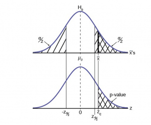
Both decision rules will result in the same decision and it is a matter of preference which one is used.

One and Two-tailed Tests

The claim would be in the alternative hypothesis. The burden of proof in hypothesis testing is carried in the alternative. This is because failing to reject the null, the status quo, must be accomplished with 90 or 95 percent significance that it cannot be maintained. Said another way, we want to have only a 5 or 10 percent probability of making a Type I error, rejecting a good null; overthrowing the status quo.

Figure 5 shows the two possible cases and the form of the null and alternative hypothesis that give rise to them.

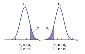
Effects of Sample Size on Test Statistic

Table 3 summarizes test statistics for varying sample sizes and population standard deviation known and unknown.

A Systematic Approach for Testing A Hypothesis

A systematic approach to hypothesis testing follows the following steps and in this order. This template will work for all hypotheses that you will ever test.

• Set up the null and alternative hypothesis. This is typically the hardest part of the process. Here the question being asked is reviewed. What parameter is being tested, a mean, a proportion, differences in means, etc. Is this a one-tailed test or two-tailed test? Remember, if someone is making a claim it will always be a one-tailed test.
• Decide the level of significance required for this particular case and determine the critical value. These can be found in the appropriate statistical table. The levels of confidence typical for the social sciences are 90, 95 and 99. However, the level of significance is a policy decision and should be based upon the risk of making a Type I error, rejecting a good null. Consider the consequences of making a Type I error.
• Take a sample(s) and calculate the relevant parameters: sample mean, standard deviation, or proportion. Using the formula for the test statistic from above in step 2, now calculate the test statistic for this particular case using the parameters you have just calculated.
• Compare the calculated test statistic and the critical value. Marking these on the graph will give a good visual picture of the situation. There are now only two situations:

a.     The test statistic is in the tail: Cannot Accept the null, the probability that this sample mean (proportion) came from the hypothesized distribution is too small to believe that it is the real home of these sample data.

b.   The test statistic is not in the tail: Cannot Reject the null, the sample data are compatible with the hypothesized population parameter.

• Reach a conclusion. It is best to articulate the conclusion two different ways. First a formal statistical conclusion such as “With a 95 % level of significance we cannot accept the null hypotheses that the population mean is equal to XX (units of measurement)”. The second statement of the conclusion is less formal and states the action, or lack of action, required. If the formal conclusion was that above, then the informal one might be, “The machine is broken and we need to shut it down and call for repairs”.

All hypotheses tested will go through this same process. The only changes are the relevant formulas and those are determined by the hypothesis required to answer the original question.

Full Hypothesis Test Examples

Tests on means.

Jeffrey, as an eight-year old, established a mean time of 16.43 seconds for swimming the 25-yard freestyle, with a standard deviation of 0.8 seconds . His dad, Frank, thought that Jeffrey could swim the 25-yard freestyle faster using goggles. Frank bought Jeffrey a new pair of expensive goggles and timed Jeffrey for 15 25-yard freestyle swims . For the 15 swims, Jeffrey’s mean time was 16 seconds. Frank thought that the goggles helped Jeffrey to swim faster than the 16.43 seconds. Conduct a hypothesis test using a preset α = 0.05.

Solution – Example 6

Set up the Hypothesis Test:

Since the problem is about a mean, this is a test of a single population mean . Set the null and alternative hypothesis:

In this case there is an implied challenge or claim. This is that the goggles will reduce the swimming time. The effect of this is to set the hypothesis as a one-tailed test. The claim will always be in the alternative hypothesis because the burden of proof always lies with the alternative. Remember that the status quo must be defeated with a high degree of confidence, in this case 95 % confidence. The null and alternative hypotheses are thus:

For Jeffrey to swim faster, his time will be less than 16.43 seconds. The “<” tells you this is left-tailed. Determine the distribution needed:

Distribution for the test statistic:

The sample size is less than 30 and we do not know the population standard deviation so this is a t-test and the proper formula is:

Our step 2, setting the level of significance, has already been determined by the problem, .05 for a 95 % significance level. It is worth thinking about the meaning of this choice. The Type I error is to conclude that Jeffrey swims the 25-yard freestyle, on average, in less than 16.43 seconds when, in fact, he actually swims the 25-yard freestyle, on average, in 16.43 seconds. (Reject the null hypothesis when the null hypothesis is true.) For this case the only concern with a Type I error would seem to be that Jeffery’s dad may fail to bet on his son’s victory because he does not have appropriate confidence in the effect of the goggles.

To find the critical value we need to select the appropriate test statistic. We have concluded that this is a t-test on the basis of the sample size and that we are interested in a population mean. We can now draw the graph of the t-distribution and mark the critical value (Figure 6). For this problem the degrees of freedom are n-1, or 14. Looking up 14 degrees of freedom at the 0.05 column of the t-table we find 1.761. This is the critical value and we can put this on our graph.

Step 3 is the calculation of the test statistic using the formula we have selected.

We find that the calculated test statistic is 2.08, meaning that the sample mean is 2.08 standard deviations away from the hypothesized mean of 16.43.

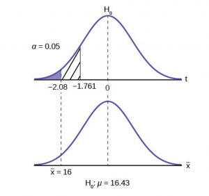
Step 4 has us compare the test statistic and the critical value and mark these on the graph. We see that the test statistic is in the tail and thus we move to step 4 and reach a conclusion. The probability that an average time of 16 minutes could come from a distribution with a population mean of 16.43 minutes is too unlikely for us to accept the null hypothesis. We cannot accept the null.

Step 5 has us state our conclusions first formally and then less formally. A formal conclusion would be stated as: “With a 95% level of significance we cannot accept the null hypothesis that the swimming time with goggles comes from a distribution with a population mean time of 16.43 minutes.” Less formally, “With 95% significance we believe that the goggles improves swimming speed”

If we wished to use the p-value system of reaching a conclusion we would calculate the statistic and take the additional step to find the probability of being 2.08 standard deviations from the mean on a t-distribution. This value is .0187. Comparing this to the α-level of .05 we see that we cannot accept the null. The p-value has been put on the graph as the shaded area beyond -2.08 and it shows that it is smaller than the hatched area which is the alpha level of 0.05. Both methods reach the same conclusion that we cannot accept the null hypothesis.

Jane has just begun her new job as on the sales force of a very competitive company. In a sample of 16 sales calls it was found that she closed the contract for an average value of $108 with a standard deviation of 12 dollars. Test at 5% significance that the population mean is at least $100 against the alternative that it is less than 100 dollars. Company policy requires that new members of the sales force must exceed an average of $100 per contract during the trial employment period. Can we conclude that Jane has met this requirement at the significance level of 95%?

Solution – Example 7

STEP 1 : Set the Null and Alternative Hypothesis.

STEP 2 : Decide the level of significance and draw the graph (Figure 7) showing the critical value.

STEP 3 : Calculate sample parameters and the test statistic.

STEP 4 : Compare test statistic and the critical values

STEP 5 : Reach a Conclusion

The test statistic is a Student’s t because the sample size is below 30; therefore, we cannot use the normal distribution. Comparing the calculated value of the test statistic and the critical value of t ( t a ) at a 5% significance level, we see that the calculated value is in the tail of the distribution. Thus, we conclude that 108 dollars per contract is significantly larger than the hypothesized value of 100 and thus we cannot accept the null hypothesis. There is evidence that supports Jane’s performance meets company standards.

Again we will follow the steps in our analysis of this problem.

Solution – Example 8

STEP 1 : Set the Null and Alternative Hypothesis. The random variable is the quantity of fluid placed in the bottles. This is a continuous random variable and the parameter we are interested in is the mean. Our hypothesis therefore is about the mean. In this case we are concerned that the machine is not filling properly. From what we are told it does not matter if the machine is over-filling or under-filling, both seem to be an equally bad error. This tells us that this is a two-tailed test: if the machine is malfunctioning it will be shutdown regardless if it is from over-filling or under-filling. The null and alternative hypotheses are thus:

STEP 2 : Decide the level of significance and draw the graph showing the critical value.

This problem has already set the level of significance at 99%. The decision seems an appropriate one and shows the thought process when setting the significance level. Management wants to be very certain, as certain as probability will allow, that they are not shutting down a machine that is not in need of repair. To draw the distribution and the critical value, we need to know which distribution to use. Because this is a continuous random variable and we are interested in the mean, and the sample size is greater than 30, the appropriate distribution is the normal distribution and the relevant critical value is 2.575 from the normal table or the t-table at 0.005 column and infinite degrees of freedom. We draw the graph and mark these points (Figure 8).

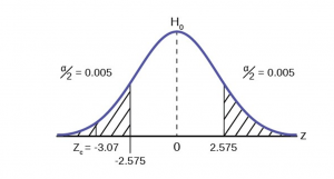
STEP 3 : Calculate sample parameters and the test statistic. The sample parameters are provided, the sample mean is 7.91 and the sample variance is .03 and the sample size is 35. We need to note that the sample variance was provided not the sample standard deviation, which is what we need for the formula. Remembering that the standard deviation is simply the square root of the variance, we therefore know the sample standard deviation, s, is 0.173. With this information we calculate the test statistic as -3.07, and mark it on the graph.

STEP 4 : Compare test statistic and the critical values Now we compare the test statistic and the critical value by placing the test statistic on the graph. We see that the test statistic is in the tail, decidedly greater than the critical value of 2.575. We note that even the very small difference between the hypothesized value and the sample value is still a large number of standard deviations. The sample mean is only 0.08 ounces different from the required level of 8 ounces, but it is 3 plus standard deviations away and thus we cannot accept the null hypothesis.

Three standard deviations of a test statistic will guarantee that the test will fail. The probability that anything is within three standard deviations is almost zero. Actually it is 0.0026 on the normal distribution, which is certainly almost zero in a practical sense. Our formal conclusion would be “ At a 99% level of significance we cannot accept the hypothesis that the sample mean came from a distribution with a mean of 8 ounces” Or less formally, and getting to the point, “At a 99% level of significance we conclude that the machine is under filling the bottles and is in need of repair”.

Media Attributions

• Type1Type2Error
• HypTestFig2
• HypTestFig3
• HypTestPValue
• OneTailTestFig5
• HypTestExam7
• HypTestExam8

Quantitative Analysis for Business Copyright © by Margo Bergman is licensed under a Creative Commons Attribution-NonCommercial-ShareAlike 4.0 International License , except where otherwise noted.

Share This Book

• Search Search Please fill out this field.

What Is Hypothesis Testing?

Step 1: define the hypothesis, step 2: set the criteria, step 3: calculate the statistic, step 4: reach a conclusion, types of errors, the bottom line.

• Trading Skills
• Trading Basic Education

Hypothesis Testing in Finance: Concept and Examples

Charlene Rhinehart is a CPA , CFE, chair of an Illinois CPA Society committee, and has a degree in accounting and finance from DePaul University.

Your investment advisor proposes you a monthly income investment plan that promises a variable return each month. You will invest in it only if you are assured of an average $180 monthly income. Your advisor also tells you that for the past 300 months, the scheme had investment returns with an average value of $190 and a standard deviation of $75. Should you invest in this scheme? Hypothesis testing comes to the aid for such decision-making.

Key Takeaways

• Hypothesis testing is a mathematical tool for confirming a financial or business claim or idea.
• Hypothesis testing is useful for investors trying to decide what to invest in and whether the instrument is likely to provide a satisfactory return.
• Despite the existence of different methodologies of hypothesis testing, the same four steps are used: define the hypothesis, set the criteria, calculate the statistic, and reach a conclusion.
• This mathematical model, like most statistical tools and models, has limitations and is prone to certain errors, necessitating investors also considering other models in conjunction with this one

Hypothesis or significance testing is a mathematical model for testing a claim, idea or hypothesis about a parameter of interest in a given population set, using data measured in a sample set. Calculations are performed on selected samples to gather more decisive information about the characteristics of the entire population, which enables a systematic way to test claims or ideas about the entire dataset.

Here is a simple example: A school principal reports that students in their school score an average of 7 out of 10 in exams. To test this “hypothesis,” we record marks of say 30 students (sample) from the entire student population of the school (say 300) and calculate the mean of that sample. We can then compare the (calculated) sample mean to the (reported) population mean and attempt to confirm the hypothesis.

To take another example, the annual return of a particular mutual fund is 8%. Assume that mutual fund has been in existence for 20 years. We take a random sample of annual returns of the mutual fund for, say, five years (sample) and calculate its mean. We then compare the (calculated) sample mean to the (claimed) population mean to verify the hypothesis.

This article assumes readers' familiarity with concepts of a normal distribution table, formula, p-value and related basics of statistics.

Different methodologies exist for hypothesis testing, but the same four basic steps are involved:

Usually, the reported value (or the claim statistics) is stated as the hypothesis and presumed to be true. For the above examples, the hypothesis will be:

• Example A: Students in the school score an average of 7 out of 10 in exams.
• Example B: The annual return of the mutual fund is 8% per annum.

This stated description constitutes the “ Null Hypothesis (H 0 ) ” and is  assumed  to be true – the way a defendant in a jury trial is presumed innocent until proven guilty by the evidence presented in court. Similarly, hypothesis testing starts by stating and assuming a “ null hypothesis ,” and then the process determines whether the assumption is likely to be true or false.

The important point to note is that we are testing the null hypothesis because there is an element of doubt about its validity. Whatever information that is against the stated null hypothesis is captured in the  Alternative Hypothesis (H 1 ).  For the above examples, the alternative hypothesis will be:

• Students score an average that is not equal to 7.
• The annual return of the mutual fund is not equal to 8% per annum.

In other words, the alternative hypothesis is a direct contradiction of the null hypothesis.

As in a trial, the jury assumes the defendant's innocence (null hypothesis). The prosecutor has to prove otherwise (alternative hypothesis). Similarly, the researcher has to prove that the null hypothesis is either true or false. If the prosecutor fails to prove the alternative hypothesis, the jury has to let the defendant go (basing the decision on the null hypothesis). Similarly, if the researcher fails to prove an alternative hypothesis (or simply does nothing), then the null hypothesis is assumed to be true.

The decision-making criteria have to be based on certain parameters of datasets.

The decision-making criteria have to be based on certain parameters of datasets and this is where the connection to normal distribution comes into the picture.

As per the standard statistics postulate  about sampling distribution , “For any sample size n, the sampling distribution of X̅ is normal if the population X from which the sample is drawn is normally distributed.” Hence, the probabilities of all other possible sample mean that one could select are normally distributed.

For e.g., determine if the average daily return, of any stock listed on XYZ stock market , around New Year's Day is greater than 2%.

H 0 : Null Hypothesis: mean = 2%

H 1 : Alternative Hypothesis: mean > 2% (this is what we want to prove)

Take the sample (say of 50 stocks out of total 500) and compute the mean of the sample.

For a normal distribution, 95% of the values lie within two standard deviations of the population mean. Hence, this normal distribution and central limit assumption for the sample dataset allows us to establish 5% as a significance level. It makes sense as, under this assumption, there is less than a 5% probability (100-95) of getting outliers that are beyond two standard deviations from the population mean. Depending upon the nature of datasets, other significance levels can be taken at 1%, 5% or 10%. For financial calculations (including behavioral finance), 5% is the generally accepted limit. If we find any calculations that go beyond the usual two standard deviations, then we have a strong case of outliers to reject the null hypothesis.  

Graphically, it is represented as follows:

In the above example, if the mean of the sample is much larger than 2% (say 3.5%), then we reject the null hypothesis. The alternative hypothesis (mean >2%) is accepted, which confirms that the average daily return of the stocks is indeed above 2%.

However, if the mean of the sample is not likely to be significantly greater than 2% (and remains at, say, around 2.2%), then we CANNOT reject the null hypothesis. The challenge comes on how to decide on such close range cases. To make a conclusion from selected samples and results, a level of significance is to be determined, which enables a conclusion to be made about the null hypothesis. The alternative hypothesis enables establishing the level of significance or the "critical value” concept for deciding on such close range cases.

According to the textbook standard definition , “A critical value is a cutoff value that defines the boundaries beyond which less than 5% of sample means can be obtained if the null hypothesis is true. Sample means obtained beyond a critical value will result in a decision to reject the null hypothesis."   In the above example, if we have defined the critical value as 2.1%, and the calculated mean comes to 2.2%, then we reject the null hypothesis. A critical value establishes a clear demarcation about acceptance or rejection.

This step involves calculating the required figure(s), known as test statistics (like mean, z-score , p-value , etc.), for the selected sample. (We'll get to these in a later section.)

With the computed value(s), decide on the null hypothesis. If the probability of getting a sample mean is less than 5%, then the conclusion is to reject the null hypothesis. Otherwise, accept and retain the null hypothesis.

There can be four possible outcomes in sample-based decision-making, with regard to the correct applicability to the entire population:

The “Correct” cases are the ones where the decisions taken on the samples are truly applicable to the entire population. The cases of errors arise when one decides to retain (or reject) the null hypothesis based on the sample calculations, but that decision does not really apply for the entire population. These cases constitute Type 1 ( alpha ) and Type 2 ( beta ) errors, as indicated in the table above.

Selecting the correct critical value allows eliminating the type-1 alpha errors or limiting them to an acceptable range.

Alpha denotes the error on the level of significance and is determined by the researcher. To maintain the standard 5% significance or confidence level for probability calculations, this is retained at 5%.

According to the applicable decision-making benchmarks and definitions:

• “This (alpha) criterion is usually set at 0.05 (a = 0.05), and we compare the alpha level to the p-value. When the probability of a Type I error is less than 5% (p < 0.05), we decide to reject the null hypothesis; otherwise, we retain the null hypothesis.”  
• The technical term used for this probability is the p-value . It is defined as “the probability of obtaining a sample outcome, given that the value stated in the null hypothesis is true. The p-value for obtaining a sample outcome is compared to the level of significance."  
• A Type II error, or beta error, is defined as the probability of incorrectly retaining the null hypothesis, when in fact it is not applicable to the entire population.  

A few more examples will demonstrate this and other calculations.

A monthly income investment scheme exists that promises variable monthly returns. An investor will invest in it only if they are assured of an average $180 monthly income. The investor has a sample of 300 months’ returns which has a mean of $190 and a standard deviation of $75. Should they invest in this scheme?

Let’s set up the problem. The investor will invest in the scheme if they are assured of the investor's desired $180 average return.

H 0 : Null Hypothesis: mean = 180

H 1 : Alternative Hypothesis: mean > 180

Method 1: Critical Value Approach

Identify a critical value X L for the sample mean, which is large enough to reject the null hypothesis – i.e. reject the null hypothesis if the sample mean >= critical value X L

P (identify a Type I alpha error) = P(reject H 0  given that H 0  is true),

This would be achieved when the sample mean exceeds the critical limits.

= P (given that H 0  is true) = alpha

Graphically, it appears as follows:

Taking alpha = 0.05 (i.e. 5% significance level), Z 0.05  = 1.645 (from the Z-table or normal distribution table)

           = > X L  = 180 +1.645*(75/sqrt(300)) = 187.12

Since the sample mean (190) is greater than the critical value (187.12), the null hypothesis is rejected, and the conclusion is that the average monthly return is indeed greater than $180, so the investor can consider investing in this scheme.

Method 2: Using Standardized Test Statistics

One can also use standardized value z.

Test Statistic, Z = (sample mean – population mean) / (std-dev / sqrt (no. of samples).

Then, the rejection region becomes the following:

Z= (190 – 180) / (75 / sqrt (300)) = 2.309

Our rejection region at 5% significance level is Z> Z 0.05  = 1.645.

Since Z= 2.309 is greater than 1.645, the null hypothesis can be rejected with a similar conclusion mentioned above.

Method 3: P-value Calculation

We aim to identify P (sample mean >= 190, when mean = 180).

= P (Z >= (190- 180) / (75 / sqrt (300))

= P (Z >= 2.309) = 0.0084 = 0.84%

The following table to infer p-value calculations concludes that there is confirmed evidence of average monthly returns being higher than 180:

A new stockbroker (XYZ) claims that their brokerage fees are lower than that of your current stock broker's (ABC). Data available from an independent research firm indicates that the mean and std-dev of all ABC broker clients are $18 and $6, respectively.

A sample of 100 clients of ABC is taken and brokerage charges are calculated with the new rates of XYZ broker. If the mean of the sample is $18.75 and std-dev is the same ($6), can any inference be made about the difference in the average brokerage bill between ABC and XYZ broker?

H 0 : Null Hypothesis: mean = 18

H 1 : Alternative Hypothesis: mean <> 18 (This is what we want to prove.)

Rejection region: Z <= - Z 2.5  and Z>=Z 2.5  (assuming 5% significance level, split 2.5 each on either side).

Z = (sample mean – mean) / (std-dev / sqrt (no. of samples))

= (18.75 – 18) / (6/(sqrt(100)) = 1.25

This calculated Z value falls between the two limits defined by:

- Z 2.5  = -1.96 and Z 2.5  = 1.96.

This concludes that there is insufficient evidence to infer that there is any difference between the rates of your existing broker and the new broker.

Alternatively, The p-value = P(Z< -1.25)+P(Z >1.25)

= 2 * 0.1056 = 0.2112 = 21.12% which is greater than 0.05 or 5%, leading to the same conclusion.

Graphically, it is represented by the following:

Criticism Points for the Hypothetical Testing Method:

• A statistical method based on assumptions
• Error-prone as detailed in terms of alpha and beta errors
• Interpretation of p-value can be ambiguous, leading to confusing results

Hypothesis testing allows a mathematical model to validate a claim or idea with a certain confidence level. However, like the majority of statistical tools and models, it is bound by a few limitations. The use of this model for making financial decisions should be considered with a critical eye, keeping all dependencies in mind. Alternate methods like  Bayesian Inference are also worth exploring for similar analysis.

Sage Publications. " Introduction to Hypothesis Testing ," Page 13.

Sage Publications. " Introduction to Hypothesis Testing ," Page 11.

Sage Publications. " Introduction to Hypothesis Testing ," Page 7.

Sage Publications. " Introduction to Hypothesis Testing ," Pages 10-11.

• Terms of Service
• Editorial Policy
• Privacy Policy
• Your Privacy Choices

Have a language expert improve your writing

Run a free plagiarism check in 10 minutes, generate accurate citations for free.

• Knowledge Base

Methodology

• How to Write a Strong Hypothesis | Steps & Examples

How to Write a Strong Hypothesis | Steps & Examples

Published on May 6, 2022 by Shona McCombes . Revised on November 20, 2023.

A hypothesis is a statement that can be tested by scientific research. If you want to test a relationship between two or more variables, you need to write hypotheses before you start your experiment or data collection .

Example: Hypothesis

Daily apple consumption leads to fewer doctor’s visits.

Table of contents

What is a hypothesis, developing a hypothesis (with example), hypothesis examples, other interesting articles, frequently asked questions about writing hypotheses.

A hypothesis states your predictions about what your research will find. It is a tentative answer to your research question that has not yet been tested. For some research projects, you might have to write several hypotheses that address different aspects of your research question.

A hypothesis is not just a guess – it should be based on existing theories and knowledge. It also has to be testable, which means you can support or refute it through scientific research methods (such as experiments, observations and statistical analysis of data).

Variables in hypotheses

Hypotheses propose a relationship between two or more types of variables .

• An independent variable is something the researcher changes or controls.
• A dependent variable is something the researcher observes and measures.

If there are any control variables , extraneous variables , or confounding variables , be sure to jot those down as you go to minimize the chances that research bias  will affect your results.

In this example, the independent variable is exposure to the sun – the assumed cause . The dependent variable is the level of happiness – the assumed effect .

Here's why students love Scribbr's proofreading services

Discover proofreading & editing

Step 1. Ask a question

Writing a hypothesis begins with a research question that you want to answer. The question should be focused, specific, and researchable within the constraints of your project.

Step 2. Do some preliminary research

Your initial answer to the question should be based on what is already known about the topic. Look for theories and previous studies to help you form educated assumptions about what your research will find.

At this stage, you might construct a conceptual framework to ensure that you’re embarking on a relevant topic . This can also help you identify which variables you will study and what you think the relationships are between them. Sometimes, you’ll have to operationalize more complex constructs.

Step 3. Formulate your hypothesis

Now you should have some idea of what you expect to find. Write your initial answer to the question in a clear, concise sentence.

4. Refine your hypothesis

You need to make sure your hypothesis is specific and testable. There are various ways of phrasing a hypothesis, but all the terms you use should have clear definitions, and the hypothesis should contain:

• The relevant variables
• The specific group being studied
• The predicted outcome of the experiment or analysis

5. Phrase your hypothesis in three ways

To identify the variables, you can write a simple prediction in  if…then form. The first part of the sentence states the independent variable and the second part states the dependent variable.

In academic research, hypotheses are more commonly phrased in terms of correlations or effects, where you directly state the predicted relationship between variables.

If you are comparing two groups, the hypothesis can state what difference you expect to find between them.

6. Write a null hypothesis

If your research involves statistical hypothesis testing , you will also have to write a null hypothesis . The null hypothesis is the default position that there is no association between the variables. The null hypothesis is written as H 0 , while the alternative hypothesis is H 1 or H a .

• H 0 : The number of lectures attended by first-year students has no effect on their final exam scores.
• H 1 : The number of lectures attended by first-year students has a positive effect on their final exam scores.

If you want to know more about the research process , methodology , research bias , or statistics , make sure to check out some of our other articles with explanations and examples.

• Sampling methods
• Simple random sampling
• Stratified sampling
• Cluster sampling
• Likert scales
• Reproducibility

 Statistics

• Null hypothesis
• Statistical power
• Probability distribution
• Effect size
• Poisson distribution

Research bias

• Optimism bias
• Cognitive bias
• Implicit bias
• Hawthorne effect
• Anchoring bias
• Explicit bias

Prevent plagiarism. Run a free check.

A hypothesis is not just a guess — it should be based on existing theories and knowledge. It also has to be testable, which means you can support or refute it through scientific research methods (such as experiments, observations and statistical analysis of data).

Null and alternative hypotheses are used in statistical hypothesis testing . The null hypothesis of a test always predicts no effect or no relationship between variables, while the alternative hypothesis states your research prediction of an effect or relationship.

Hypothesis testing is a formal procedure for investigating our ideas about the world using statistics. It is used by scientists to test specific predictions, called hypotheses , by calculating how likely it is that a pattern or relationship between variables could have arisen by chance.

Cite this Scribbr article

If you want to cite this source, you can copy and paste the citation or click the “Cite this Scribbr article” button to automatically add the citation to our free Citation Generator.

McCombes, S. (2023, November 20). How to Write a Strong Hypothesis | Steps & Examples. Scribbr. Retrieved April 9, 2024, from https://www.scribbr.com/methodology/hypothesis/

Is this article helpful?

Shona McCombes

Other students also liked, construct validity | definition, types, & examples, what is a conceptual framework | tips & examples, operationalization | a guide with examples, pros & cons, what is your plagiarism score.

What is Hypothesis Testing in Statistics? Types and Examples

Varun Saharawat is a seasoned professional in the fields of SEO and content writing. With a profound knowledge of the intricate aspects of these disciplines, Varun has established himself as a valuable asset in the world of digital marketing and online content creation.

Hypothesis testing in statistics involves testing an assumption about a population parameter using sample data. Learners can download Hypothesis Testing PDF to get instant access to all information!

What exactly is hypothesis testing, and how does it work in statistics? Can I find practical examples and understand the different types from this blog?

Hypothesis Testing : Ever wonder how researchers determine if a new medicine actually works or if a new marketing campaign effectively drives sales? They use hypothesis testing! It is at the core of how scientific studies, business experiments and surveys determine if their results are statistically significant or just due to chance.

Hypothesis testing allows us to make evidence-based decisions by quantifying uncertainty and providing a structured process to make data-driven conclusions rather than guessing. In this post, we will discuss hypothesis testing types, examples, and processes!

Table of Contents

Hypothesis Testing

Hypothesis testing is a statistical method used to evaluate the validity of a hypothesis using sample data. It involves assessing whether observed data provide enough evidence to reject a specific hypothesis about a population parameter. 

Hypothesis Testing in Data Science

Hypothesis testing in data science is a statistical method used to evaluate two mutually exclusive population statements based on sample data. The primary goal is to determine which statement is more supported by the observed data.

Hypothesis testing assists in supporting the certainty of findings in research and data science projects. This statistical inference aids in making decisions about population parameters using sample data. For those who are looking to deepen their knowledge in data science and expand their skillset, we highly recommend checking out Master Generative AI: Data Science Course by Physics Wallah .

Also Read: What is Encapsulation Explain in Details

What is the Hypothesis Testing Procedure in Data Science?

The hypothesis testing procedure in data science involves a structured approach to evaluating hypotheses using statistical methods. Here’s a step-by-step breakdown of the typical procedure:

1) State the Hypotheses:

• Null Hypothesis (H0): This is the default assumption or a statement of no effect or difference. It represents what you aim to test against.
• Alternative Hypothesis (Ha): This is the opposite of the null hypothesis and represents what you want to prove.

2) Choose a Significance Level (α):

• Decide on a threshold (commonly 0.05) beyond which you will reject the null hypothesis. This is your significance level.

3) Select the Appropriate Test:

• Depending on your data type (e.g., continuous, categorical) and the nature of your research question, choose the appropriate statistical test (e.g., t-test, chi-square test, ANOVA, etc.).

4) Collect Data:

• Gather data from your sample or population, ensuring that it’s representative and sufficiently large (or as per your experimental design).

5)Compute the Test Statistic:

• Using your data and the chosen statistical test, compute the test statistic that summarizes the evidence against the null hypothesis.

6) Determine the Critical Value or P-value:

• Based on your significance level and the test statistic’s distribution, determine the critical value from a statistical table or compute the p-value.

7) Make a Decision:

• If the p-value is less than α: Reject the null hypothesis.
• If the p-value is greater than or equal to α: Fail to reject the null hypothesis.

8) Draw Conclusions:

• Based on your decision, draw conclusions about your research question or hypothesis. Remember, failing to reject the null hypothesis doesn’t prove it true; it merely suggests that you don’t have sufficient evidence to reject it.

9) Report Findings:

• Document your findings, including the test statistic, p-value, conclusion, and any other relevant details. Ensure clarity so that others can understand and potentially replicate your analysis.

Also Read: Binary Search Algorithm

How Hypothesis Testing Works?

Hypothesis testing is a fundamental concept in statistics that aids analysts in making informed decisions based on sample data about a larger population. The process involves setting up two contrasting hypotheses, the null hypothesis and the alternative hypothesis, and then using statistical methods to determine which hypothesis provides a more plausible explanation for the observed data.

The Core Principles:

• The Null Hypothesis (H0): This serves as the default assumption or status quo. Typically, it posits that there is no effect or no difference, often represented by an equality statement regarding population parameters. For instance, it might state that a new drug’s effect is no different from a placebo.
• The Alternative Hypothesis (H1 or Ha): This is the counter assumption or what researchers aim to prove. It’s the opposite of the null hypothesis, indicating that there is an effect, a change, or a difference in the population parameters. Using the drug example, the alternative hypothesis would suggest that the new drug has a different effect than the placebo.

Testing the Hypotheses:

Once these hypotheses are established, analysts gather data from a sample and conduct statistical tests. The objective is to determine whether the observed results are statistically significant enough to reject the null hypothesis in favor of the alternative.

Examples to Clarify the Concept:

• Null Hypothesis (H0): The sanitizer’s average efficacy is 95%.
• By conducting tests, if evidence suggests that the sanitizer’s efficacy is significantly less than 95%, we reject the null hypothesis.
• Null Hypothesis (H0): The coin is fair, meaning the probability of heads and tails is equal.
• Through experimental trials, if results consistently show a skewed outcome, indicating a significantly different probability for heads and tails, the null hypothesis might be rejected.

What are the 3 types of Hypothesis Test?

Hypothesis testing is a cornerstone in statistical analysis, providing a framework to evaluate the validity of assumptions or claims made about a population based on sample data. Within this framework, several specific tests are utilized based on the nature of the data and the question at hand. Here’s a closer look at the three fundamental types of hypothesis tests:

The z-test is a statistical method primarily employed when comparing means from two datasets, particularly when the population standard deviation is known. Its main objective is to ascertain if the means are statistically equivalent. 

A crucial prerequisite for the z-test is that the sample size should be relatively large, typically 30 data points or more. This test aids researchers and analysts in determining the significance of a relationship or discovery, especially in scenarios where the data’s characteristics align with the assumptions of the z-test.

The t-test is a versatile statistical tool used extensively in research and various fields to compare means between two groups. It’s particularly valuable when the population standard deviation is unknown or when dealing with smaller sample sizes. 

By evaluating the means of two groups, the t-test helps ascertain if a particular treatment, intervention, or variable significantly impacts the population under study. Its flexibility and robustness make it a go-to method in scenarios ranging from medical research to business analytics.

3. Chi-Square Test:

The Chi-Square test stands distinct from the previous tests, primarily focusing on categorical data rather than means. This statistical test is instrumental when analyzing categorical variables to determine if observed data aligns with expected outcomes as posited by the null hypothesis. 

By assessing the differences between observed and expected frequencies within categorical data, the Chi-Square test offers insights into whether discrepancies are statistically significant. Whether used in social sciences to evaluate survey responses or in quality control to assess product defects, the Chi-Square test remains pivotal for hypothesis testing in diverse scenarios.

Also Read: Python vs Java: Which is Best for Machine learning algorithm

Hypothesis Testing in Statistics

Hypothesis testing is a fundamental concept in statistics used to make decisions or inferences about a population based on a sample of data. The process involves setting up two competing hypotheses, the null hypothesis H 0​ and the alternative hypothesis H 1​. 

Through various statistical tests, such as the t-test, z-test, or Chi-square test, analysts evaluate sample data to determine whether there’s enough evidence to reject the null hypothesis in favor of the alternative. The aim is to draw conclusions about population parameters or to test theories, claims, or hypotheses.

Hypothesis Testing in Research

In research, hypothesis testing serves as a structured approach to validate or refute theories or claims. Researchers formulate a clear hypothesis based on existing literature or preliminary observations. They then collect data through experiments, surveys, or observational studies. 

Using statistical methods, researchers analyze this data to determine if there’s sufficient evidence to reject the null hypothesis. By doing so, they can draw meaningful conclusions, make predictions, or recommend actions based on empirical evidence rather than mere speculation.

Hypothesis Testing in R

R, a powerful programming language and environment for statistical computing and graphics, offers a wide array of functions and packages specifically designed for hypothesis testing. Here’s how hypothesis testing is conducted in R:

• Data Collection : Before conducting any test, you need to gather your data and ensure it’s appropriately structured in R.
• Choose the Right Test : Depending on your research question and data type, select the appropriate hypothesis test. For instance, use the t.test() function for a t-test or chisq.test() for a Chi-square test.
• Set Hypotheses : Define your null and alternative hypotheses. Using R’s syntax, you can specify these hypotheses and run the corresponding test.
• Execute the Test : Utilize built-in functions in R to perform the hypothesis test on your data. For instance, if you want to compare two means, you can use the t.test() function, providing the necessary arguments like the data vectors and type of t-test (one-sample, two-sample, paired, etc.).
• Interpret Results : Once the test is executed, R will provide output, including test statistics, p-values, and confidence intervals. Based on these results and a predetermined significance level (often 0.05), you can decide whether to reject the null hypothesis.
• Visualization : R’s graphical capabilities allow users to visualize data distributions, confidence intervals, or test statistics, aiding in the interpretation and presentation of results.

Hypothesis testing is an integral part of statistics and research, offering a systematic approach to validate hypotheses. Leveraging R’s capabilities, researchers and analysts can efficiently conduct and interpret various hypothesis tests, ensuring robust and reliable conclusions from their data.

Do Data Scientists do Hypothesis Testing?

Yes, data scientists frequently engage in hypothesis testing as part of their analytical toolkit. Hypothesis testing is a foundational statistical technique used to make data-driven decisions, validate assumptions, and draw conclusions from data. Here’s how data scientists utilize hypothesis testing:

• Validating Assumptions : Before diving into complex analyses or building predictive models, data scientists often need to verify certain assumptions about the data. Hypothesis testing provides a structured approach to test these assumptions, ensuring that subsequent analyses or models are valid.
• Feature Selection : In machine learning and predictive modeling, data scientists use hypothesis tests to determine which features (or variables) are most relevant or significant in predicting a particular outcome. By testing hypotheses related to feature importance or correlation, they can streamline the modeling process and enhance prediction accuracy.
• A/B Testing : A/B testing is a common technique in marketing, product development, and user experience design. Data scientists employ hypothesis testing to compare two versions (A and B) of a product, feature, or marketing strategy to determine which performs better in terms of a specified metric (e.g., conversion rate, user engagement).
• Research and Exploration : In exploratory data analysis (EDA) or when investigating specific research questions, data scientists formulate hypotheses to test certain relationships or patterns within the data. By conducting hypothesis tests, they can validate these relationships, uncover insights, and drive data-driven decision-making.
• Model Evaluation : After building machine learning or statistical models, data scientists use hypothesis testing to evaluate the model’s performance, assess its predictive power, or compare different models. For instance, hypothesis tests like the t-test or F-test can help determine if a new model significantly outperforms an existing one based on certain metrics.
• Business Decision-making : Beyond technical analyses, data scientists employ hypothesis testing to support business decisions. Whether it’s evaluating the effectiveness of a marketing campaign, assessing customer preferences, or optimizing operational processes, hypothesis testing provides a rigorous framework to validate assumptions and guide strategic initiatives.

Hypothesis Testing Examples and Solutions

Let’s delve into some common examples of hypothesis testing and provide solutions or interpretations for each scenario.

Example: Testing the Mean

Scenario : A coffee shop owner believes that the average waiting time for customers during peak hours is 5 minutes. To test this, the owner takes a random sample of 30 customer waiting times and wants to determine if the average waiting time is indeed 5 minutes.

Hypotheses :

• H 0​ (Null Hypothesis): 5 μ =5 minutes (The average waiting time is 5 minutes)
• H 1​ (Alternative Hypothesis): 5 μ =5 minutes (The average waiting time is not 5 minutes)

Solution : Using a t-test (assuming population variance is unknown), calculate the t-statistic based on the sample mean, sample standard deviation, and sample size. Then, determine the p-value and compare it with a significance level (e.g., 0.05) to decide whether to reject the null hypothesis.

Example: A/B Testing in Marketing

Scenario : An e-commerce company wants to determine if changing the color of a “Buy Now” button from blue to green increases the conversion rate.

• H 0​: Changing the button color does not affect the conversion rate.
• H 1​: Changing the button color affects the conversion rate.

Solution : Split website visitors into two groups: one sees the blue button (control group), and the other sees the green button (test group). Track the conversion rates for both groups over a specified period. Then, use a chi-square test or z-test (for large sample sizes) to determine if there’s a statistically significant difference in conversion rates between the two groups.

Hypothesis Testing Formula

The formula for hypothesis testing typically depends on the type of test (e.g., z-test, t-test, chi-square test) and the nature of the data (e.g., mean, proportion, variance). Below are the basic formulas for some common hypothesis tests:

Z-Test for Population Mean :

Z=(σ/n​)(xˉ−μ0​)​

• ˉ x ˉ = Sample mean
• 0 μ 0​ = Population mean under the null hypothesis
• σ = Population standard deviation
• n = Sample size

T-Test for Population Mean :

t= (s/ n ​ ) ( x ˉ −μ 0 ​ ) ​ 

s = Sample standard deviation 

Chi-Square Test for Goodness of Fit :

χ2=∑Ei​(Oi​−Ei​)2​

• Oi ​ = Observed frequency
• Ei ​ = Expected frequency

Also Read: Full Form of OOPS

Hypothesis Testing Calculator

While you can perform hypothesis testing manually using the above formulas and statistical tables, many online tools and software packages simplify this process. Here’s how you might use a calculator or software:

• Z-Test and T-Test Calculators : These tools typically require you to input sample statistics (like sample mean, population mean, standard deviation, and sample size). Once you input these values, the calculator will provide you with the test statistic (Z or t) and a p-value.
• Chi-Square Calculator : For chi-square tests, you’d input observed and expected frequencies for different categories or groups. The calculator then computes the chi-square statistic and provides a p-value.
• Software Packages (e.g., R, Python with libraries like scipy, or statistical software like SPSS) : These platforms offer more comprehensive tools for hypothesis testing. You can run various tests, get detailed outputs, and even perform advanced analyses, including regression models, ANOVA, and more.

When using any calculator or software, always ensure you understand the underlying assumptions of the test, interpret the results correctly, and consider the broader context of your research or analysis.

Hypothesis Testing FAQs

What are the key components of a hypothesis test.

The key components include: Null Hypothesis (H0): A statement of no effect or no difference. Alternative Hypothesis (H1 or Ha): A statement that contradicts the null hypothesis. Test Statistic: A value computed from the sample data to test the null hypothesis. Significance Level (α): The threshold for rejecting the null hypothesis. P-value: The probability of observing the given data, assuming the null hypothesis is true.

What is the significance level in hypothesis testing?

The significance level (often denoted as α) is the probability threshold used to determine whether to reject the null hypothesis. Commonly used values for α include 0.05, 0.01, and 0.10, representing a 5%, 1%, or 10% chance of rejecting the null hypothesis when it's actually true.

How do I choose between a one-tailed and two-tailed test?

The choice between one-tailed and two-tailed tests depends on your research question and hypothesis. Use a one-tailed test when you're specifically interested in one direction of an effect (e.g., greater than or less than). Use a two-tailed test when you want to determine if there's a significant difference in either direction.

What is a p-value, and how is it interpreted?

The p-value is a probability value that helps determine the strength of evidence against the null hypothesis. A low p-value (typically ≤ 0.05) suggests that the observed data is inconsistent with the null hypothesis, leading to its rejection. Conversely, a high p-value suggests that the data is consistent with the null hypothesis, leading to no rejection.

Can hypothesis testing prove a hypothesis true?

No, hypothesis testing cannot prove a hypothesis true. Instead, it helps assess the likelihood of observing a given set of data under the assumption that the null hypothesis is true. Based on this assessment, you either reject or fail to reject the null hypothesis.

• Top 10 Tech Skills to Master in 2024

I have compiled a list of in-demand top 10 Tech Skills to master in 2024 to help you navigate the…

• Top 30 Excel Formulas And Functions You Should Know

Microsoft Excel is the most common instrument for working with data and their structures. A handful of people probably haven’t…

• Best Web Designing: Top 10 Website Designs to Inspire You in 2024

Great web design is essential when it comes to any online business presence. Find best web designing options, ideas, and…

Related Articles

• PW Skills Vishwas Diwas: List of Affordable Courses in Offer
• PW Skills Vishwas Diwas: List of Premium Courses Available on Discount Offers 2024
• Top 50 Manual Testing Interview Questions and Answers
• What is AWS DevOps? | Architecture, Tools, and Benefits in 2024
• SQL Interview Questions CHEAT SHEET (2024)
• Top 30+ Angular Interview Questions and Answers for 2024
• Top 10 Online Computer Programming Courses To Enroll In 2024

• Privacy Policy

Buy Me a Coffee

Home » What is a Hypothesis – Types, Examples and Writing Guide

What is a Hypothesis – Types, Examples and Writing Guide

Table of Contents

Definition:

Hypothesis is an educated guess or proposed explanation for a phenomenon, based on some initial observations or data. It is a tentative statement that can be tested and potentially proven or disproven through further investigation and experimentation.

Hypothesis is often used in scientific research to guide the design of experiments and the collection and analysis of data. It is an essential element of the scientific method, as it allows researchers to make predictions about the outcome of their experiments and to test those predictions to determine their accuracy.

Types of Hypothesis

Types of Hypothesis are as follows:

Research Hypothesis

A research hypothesis is a statement that predicts a relationship between variables. It is usually formulated as a specific statement that can be tested through research, and it is often used in scientific research to guide the design of experiments.

Null Hypothesis

The null hypothesis is a statement that assumes there is no significant difference or relationship between variables. It is often used as a starting point for testing the research hypothesis, and if the results of the study reject the null hypothesis, it suggests that there is a significant difference or relationship between variables.

Alternative Hypothesis

An alternative hypothesis is a statement that assumes there is a significant difference or relationship between variables. It is often used as an alternative to the null hypothesis and is tested against the null hypothesis to determine which statement is more accurate.

Directional Hypothesis

A directional hypothesis is a statement that predicts the direction of the relationship between variables. For example, a researcher might predict that increasing the amount of exercise will result in a decrease in body weight.

Non-directional Hypothesis

A non-directional hypothesis is a statement that predicts the relationship between variables but does not specify the direction. For example, a researcher might predict that there is a relationship between the amount of exercise and body weight, but they do not specify whether increasing or decreasing exercise will affect body weight.

Statistical Hypothesis

A statistical hypothesis is a statement that assumes a particular statistical model or distribution for the data. It is often used in statistical analysis to test the significance of a particular result.

Composite Hypothesis

A composite hypothesis is a statement that assumes more than one condition or outcome. It can be divided into several sub-hypotheses, each of which represents a different possible outcome.

Empirical Hypothesis

An empirical hypothesis is a statement that is based on observed phenomena or data. It is often used in scientific research to develop theories or models that explain the observed phenomena.

Simple Hypothesis

A simple hypothesis is a statement that assumes only one outcome or condition. It is often used in scientific research to test a single variable or factor.

Complex Hypothesis

A complex hypothesis is a statement that assumes multiple outcomes or conditions. It is often used in scientific research to test the effects of multiple variables or factors on a particular outcome.

Applications of Hypothesis

Hypotheses are used in various fields to guide research and make predictions about the outcomes of experiments or observations. Here are some examples of how hypotheses are applied in different fields:

• Science : In scientific research, hypotheses are used to test the validity of theories and models that explain natural phenomena. For example, a hypothesis might be formulated to test the effects of a particular variable on a natural system, such as the effects of climate change on an ecosystem.
• Medicine : In medical research, hypotheses are used to test the effectiveness of treatments and therapies for specific conditions. For example, a hypothesis might be formulated to test the effects of a new drug on a particular disease.
• Psychology : In psychology, hypotheses are used to test theories and models of human behavior and cognition. For example, a hypothesis might be formulated to test the effects of a particular stimulus on the brain or behavior.
• Sociology : In sociology, hypotheses are used to test theories and models of social phenomena, such as the effects of social structures or institutions on human behavior. For example, a hypothesis might be formulated to test the effects of income inequality on crime rates.
• Business : In business research, hypotheses are used to test the validity of theories and models that explain business phenomena, such as consumer behavior or market trends. For example, a hypothesis might be formulated to test the effects of a new marketing campaign on consumer buying behavior.
• Engineering : In engineering, hypotheses are used to test the effectiveness of new technologies or designs. For example, a hypothesis might be formulated to test the efficiency of a new solar panel design.

How to write a Hypothesis

Here are the steps to follow when writing a hypothesis:

Identify the Research Question

The first step is to identify the research question that you want to answer through your study. This question should be clear, specific, and focused. It should be something that can be investigated empirically and that has some relevance or significance in the field.

Conduct a Literature Review

Before writing your hypothesis, it’s essential to conduct a thorough literature review to understand what is already known about the topic. This will help you to identify the research gap and formulate a hypothesis that builds on existing knowledge.

Determine the Variables

The next step is to identify the variables involved in the research question. A variable is any characteristic or factor that can vary or change. There are two types of variables: independent and dependent. The independent variable is the one that is manipulated or changed by the researcher, while the dependent variable is the one that is measured or observed as a result of the independent variable.

Formulate the Hypothesis

Based on the research question and the variables involved, you can now formulate your hypothesis. A hypothesis should be a clear and concise statement that predicts the relationship between the variables. It should be testable through empirical research and based on existing theory or evidence.

Write the Null Hypothesis

The null hypothesis is the opposite of the alternative hypothesis, which is the hypothesis that you are testing. The null hypothesis states that there is no significant difference or relationship between the variables. It is important to write the null hypothesis because it allows you to compare your results with what would be expected by chance.

Refine the Hypothesis

After formulating the hypothesis, it’s important to refine it and make it more precise. This may involve clarifying the variables, specifying the direction of the relationship, or making the hypothesis more testable.

Examples of Hypothesis

Here are a few examples of hypotheses in different fields:

• Psychology : “Increased exposure to violent video games leads to increased aggressive behavior in adolescents.”
• Biology : “Higher levels of carbon dioxide in the atmosphere will lead to increased plant growth.”
• Sociology : “Individuals who grow up in households with higher socioeconomic status will have higher levels of education and income as adults.”
• Education : “Implementing a new teaching method will result in higher student achievement scores.”
• Marketing : “Customers who receive a personalized email will be more likely to make a purchase than those who receive a generic email.”
• Physics : “An increase in temperature will cause an increase in the volume of a gas, assuming all other variables remain constant.”
• Medicine : “Consuming a diet high in saturated fats will increase the risk of developing heart disease.”

Purpose of Hypothesis

The purpose of a hypothesis is to provide a testable explanation for an observed phenomenon or a prediction of a future outcome based on existing knowledge or theories. A hypothesis is an essential part of the scientific method and helps to guide the research process by providing a clear focus for investigation. It enables scientists to design experiments or studies to gather evidence and data that can support or refute the proposed explanation or prediction.

The formulation of a hypothesis is based on existing knowledge, observations, and theories, and it should be specific, testable, and falsifiable. A specific hypothesis helps to define the research question, which is important in the research process as it guides the selection of an appropriate research design and methodology. Testability of the hypothesis means that it can be proven or disproven through empirical data collection and analysis. Falsifiability means that the hypothesis should be formulated in such a way that it can be proven wrong if it is incorrect.

In addition to guiding the research process, the testing of hypotheses can lead to new discoveries and advancements in scientific knowledge. When a hypothesis is supported by the data, it can be used to develop new theories or models to explain the observed phenomenon. When a hypothesis is not supported by the data, it can help to refine existing theories or prompt the development of new hypotheses to explain the phenomenon.

When to use Hypothesis

Here are some common situations in which hypotheses are used:

• In scientific research , hypotheses are used to guide the design of experiments and to help researchers make predictions about the outcomes of those experiments.
• In social science research , hypotheses are used to test theories about human behavior, social relationships, and other phenomena.
• I n business , hypotheses can be used to guide decisions about marketing, product development, and other areas. For example, a hypothesis might be that a new product will sell well in a particular market, and this hypothesis can be tested through market research.

Characteristics of Hypothesis

Here are some common characteristics of a hypothesis:

• Testable : A hypothesis must be able to be tested through observation or experimentation. This means that it must be possible to collect data that will either support or refute the hypothesis.
• Falsifiable : A hypothesis must be able to be proven false if it is not supported by the data. If a hypothesis cannot be falsified, then it is not a scientific hypothesis.
• Clear and concise : A hypothesis should be stated in a clear and concise manner so that it can be easily understood and tested.
• Based on existing knowledge : A hypothesis should be based on existing knowledge and research in the field. It should not be based on personal beliefs or opinions.
• Specific : A hypothesis should be specific in terms of the variables being tested and the predicted outcome. This will help to ensure that the research is focused and well-designed.
• Tentative: A hypothesis is a tentative statement or assumption that requires further testing and evidence to be confirmed or refuted. It is not a final conclusion or assertion.
• Relevant : A hypothesis should be relevant to the research question or problem being studied. It should address a gap in knowledge or provide a new perspective on the issue.

Advantages of Hypothesis

Hypotheses have several advantages in scientific research and experimentation:

• Guides research: A hypothesis provides a clear and specific direction for research. It helps to focus the research question, select appropriate methods and variables, and interpret the results.
• Predictive powe r: A hypothesis makes predictions about the outcome of research, which can be tested through experimentation. This allows researchers to evaluate the validity of the hypothesis and make new discoveries.
• Facilitates communication: A hypothesis provides a common language and framework for scientists to communicate with one another about their research. This helps to facilitate the exchange of ideas and promotes collaboration.
• Efficient use of resources: A hypothesis helps researchers to use their time, resources, and funding efficiently by directing them towards specific research questions and methods that are most likely to yield results.
• Provides a basis for further research: A hypothesis that is supported by data provides a basis for further research and exploration. It can lead to new hypotheses, theories, and discoveries.
• Increases objectivity: A hypothesis can help to increase objectivity in research by providing a clear and specific framework for testing and interpreting results. This can reduce bias and increase the reliability of research findings.

Limitations of Hypothesis

Some Limitations of the Hypothesis are as follows:

• Limited to observable phenomena: Hypotheses are limited to observable phenomena and cannot account for unobservable or intangible factors. This means that some research questions may not be amenable to hypothesis testing.
• May be inaccurate or incomplete: Hypotheses are based on existing knowledge and research, which may be incomplete or inaccurate. This can lead to flawed hypotheses and erroneous conclusions.
• May be biased: Hypotheses may be biased by the researcher’s own beliefs, values, or assumptions. This can lead to selective interpretation of data and a lack of objectivity in research.
• Cannot prove causation: A hypothesis can only show a correlation between variables, but it cannot prove causation. This requires further experimentation and analysis.
• Limited to specific contexts: Hypotheses are limited to specific contexts and may not be generalizable to other situations or populations. This means that results may not be applicable in other contexts or may require further testing.
• May be affected by chance : Hypotheses may be affected by chance or random variation, which can obscure or distort the true relationship between variables.

About the author

Muhammad Hassan

Researcher, Academic Writer, Web developer

You may also like

Data Collection – Methods Types and Examples

Delimitations in Research – Types, Examples and...

Research Process – Steps, Examples and Tips

Research Design – Types, Methods and Examples

Institutional Review Board – Application Sample...

Evaluating Research – Process, Examples and...

• International edition
• Australia edition
• Europe edition

Labor targets unfair company mergers in competition policy overhaul

‘Reforms that address the decline in competition can deliver big economic benefits,’ treasurer to tell ACCC

• Follow our Australia news live blog for latest updates
• Get our morning and afternoon news emails , free app or daily news podcast

Companies will be required to notify the competition watchdog of mergers of a certain size in a major revamp of Australia’s competition laws designed to reduce unfair market concentration.

On Wednesday the treasurer, Jim Chalmers , will announce that the government will overhaul the voluntary system that has left the Australian Competition and Consumer Commission flying blind when scrutinising mergers, because the regulator is only informed of about a quarter of mergers.

But despite the ACCC asking for a new approval test, the Albanese government won’t be reversing the onus of proof to require companies to prove the proposed deal wouldn’t be likely to substantially lessen competition.

Sign up for Guardian Australia’s free morning and afternoon email newsletters for your daily news roundup

Instead it will tweak the merger test and bring three years of transactions within the scope of mandatory notification to prevent serial or creeping acquisitions flying under the radar.

Chalmers will announce the merger law reforms at the ACCC’s Bannerman competition lecture, arguing that the changes will help “differentiate between harmful and beneficial mergers”.

In an advance copy of the speech seen by Guardian Australia, Chalmers says Australia’s competitiveness has been declining since the 2000s with “increasing market concentration across industries”.

“Over recent decades, the mark-ups that businesses apply to goods and services have increased by more than 2 percentage points,” he says. “Reforms that address the decline in competition can deliver big economic benefits.”

Chalmers says the government wants to tackle mergers that “can cause serious economic harm” because “they’re solely focused on squeezing out competitors to capture a larger percentage of the market” rather than lifting productivity.

“This can strangle innovation, reduce productivity in our economy and punish consumers with reduced choice.”

Chalmers says Australia’s merger laws are “no longer fit for purpose” because the ACCC “isn’t properly equipped to detect and act against anti-competitive mergers”.

Only 330 mergers are scrutinised a year, on average, but 1,400 mergers were recorded last year.

“But we don’t know whether these are the right 330, or the mergers with the greatest potential to cause harm,” Chalmers says.

The ACCC chair, Gina Cass-Gottlieb, says: “We welcome the treasurer’s announcement today that the government will move to strengthen Australia’s merger laws, which will benefit Australian consumers and businesses of all sizes, as well as the wider economy.

“Higher prices, less choice and less innovation can result from weakened competition. Stronger merger laws are critical to ensure anti-competitive mergers do not proceed.”

Under the new system “mergers above monetary thresholds and which would significantly change market concentration will need to be notified to the ACCC and be approved before proceeding”, Chalmers says.

The thresholds – which will include a measure of market share – will be determined in 2024 before the new system begins in January 2026.

after newsletter promotion

The proposal paper says “all mergers within the previous three years by the acquirer or the target” will count towards the threshold.

Australia’s competition laws have come under increased focus due to concerns market concentration is seeing consumers ripped off. The former ACCC chair Rod Sims has said the existing test that a merger will substantially lessen competition is nearly impossible to prove.

The ACCC had asked for a new approval test , stating that a “merger can only proceed if the decision maker (the ACCC or tribunal on review) is satisfied that it is not likely to substantially lessen competition”.

In its submission the ACCC said this would mean “where the material before the decision maker does not positively satisfy it that there is no likely substantial lessening of competition, a merger will not be approved”.

It rejected the claim this amounted to “a reversal of the ‘onus of proof’ as this is an administrative decision being considered outside of the court context”.

According to the government response in the proposal paper the merger test will be strengthened by specifying that substantially lessening competition would include “if the merger creates, strengthens or entrenches a position of substantial market power in any market”.

Chalmers argues that “the biggest reforms to merger settings in almost 50 years” will help create “a stronger, more competitive and more productive economy”.

In other changes, there will be a public register of all mergers and acquisitions notified to the ACCC, and the watchdog will become the “the single decision maker on all mergers”.

Mergers the ACCC says will pose no threat to competition will be approved within 30 days.

The government will also introduce cost recovery fees for assessing mergers, which treasury estimates will “be between $50,000 to $100,000 for most mergers but small businesses will be exempt”, Chalmers says.

• Australian politics
• Australian economy
• Jim Chalmers (Australian politician)
• Australian Competition and Consumer Commission (ACCC)

Most viewed