
Linear Programming and Its Applications pp 140–184 Cite as

Transportation and Assignment Problems
- James K. Strayer 2
1295 Accesses
Part of the book series: Undergraduate Texts in Mathematics ((UTM))
Transportation and assignment problems are traditional examples of linear programming problems. Although these problems are solvable by using the techniques of Chapters 2–4 directly, the solution procedure is cumbersome; hence, we develop much more efficient algorithms for handling these problems. In the case of transportation problems, the algorithm is essentially a disguised form of the dual simplex algorithm of 4§2. Assignment problems, which are special cases of transportation problems, pose difficulties for the transportation algorithm and require the development of an algorithm which takes advantage of the simpler nature of these problems.
This is a preview of subscription content, log in via an institution .
Buying options
- Available as PDF
- Read on any device
- Instant download
- Own it forever
- Compact, lightweight edition
- Dispatched in 3 to 5 business days
- Free shipping worldwide - see info
- Durable hardcover edition
Tax calculation will be finalised at checkout
Purchases are for personal use only
Unable to display preview. Download preview PDF.
Author information
Authors and affiliations.
Department of Mathematics, Lock Haven University, Lock Haven, PA, 17745, USA
James K. Strayer
You can also search for this author in PubMed Google Scholar
Rights and permissions
Reprints and permissions
Copyright information
© 1989 Springer Science+Business Media New York
About this chapter
Cite this chapter.
Strayer, J.K. (1989). Transportation and Assignment Problems. In: Linear Programming and Its Applications. Undergraduate Texts in Mathematics. Springer, New York, NY. https://doi.org/10.1007/978-1-4612-1009-2_7
Download citation
DOI : https://doi.org/10.1007/978-1-4612-1009-2_7
Publisher Name : Springer, New York, NY
Print ISBN : 978-1-4612-6982-3
Online ISBN : 978-1-4612-1009-2
eBook Packages : Springer Book Archive
Share this chapter
Anyone you share the following link with will be able to read this content:
Sorry, a shareable link is not currently available for this article.
Provided by the Springer Nature SharedIt content-sharing initiative
- Publish with us
Policies and ethics
- Find a journal
- Track your research

Snapsolve any problem by taking a picture. Try it in the Numerade app?
Introduction to Operations Research
Frederick s. hillier, gerald j. lieberman, the transportation and assignment problems - all with video answers.

Chapter Questions
The Childfair Company has three plants producing child push chairs that are to be shipped to four distribution centers. Plants 1,2 , and 3 produce 12,17 , and 11 shipments per month, respectively. Each distribution center needs to receive 10 shipments per month. The distance from each plant to the respective distributing centers is given to the right: The freight cost for each shipment is $\$ 100$ plus 50 cents per mile. How much should be shipped from each plant to each of the distribution centers to minimize the total shipping cost? (a) Formulate this problem as a transportation problem by constructing the appropriate parameter table. (b) Draw the network representation of this problem. C (c) Obtain an optimal solution.

Tom would like 3 pints of home brew today and an additional 4 pints of home brew tomorrow. Dick is willing to sell a maximum of 5 pints total at a price of $\$ 3.00$ per pint today and $\$ 2.70$ per pint tomorrow. Harry is willing to sell a maximum of 4 pints total at a price of $\$ 2.90$ per pint today and $\$ 2.80$ per pint tomorrow. Tom wishes to know what his purchases should be to minimize his cost while satisfying his thirst requirements. (a) Formulate a linear programming model for this problem, and construct the initial simplex tableau (see Chaps. 3 and 4). (b) Formulate this problem as a transportation problem by constructing the appropriate parameter table. C (c) Obtain an optimal solution.
The Versatech Corporation has decided to produce three new products. Five branch plants now have excess product capacity. The unit manufacturing cost of the first product would be $\$ 31, \$ 29$, $\$ 32, \$ 28$, and $\$ 29$ in Plants $1,2,3,4$, and 5 , respectively. The unit manufacturing cost of the second product would be $\$ 45, \$ 41, \$ 46$, $\$ 42$, and $\$ 43$ in Plants $1,2,3,4$, and 5, respectively. The unit manufacturing cost of the third product would be $\$ 38, \$ 35$, and $\$ 40$ in Plants 1,2 , and 3 , respectively, whereas Plants 4 and 5 do not have the capability for producing this product. Sales forecasts indicate that $600,1,000$, and 800 units of products 1,2 , and 3 , respectively, should be produced per day. Plants $1,2,3,4$, and 5 have the capacity to produce $400,600,400,600$, and 1,000 units daily, respectively, regardless of the product or combination of products involved. Assume that any plant having the capability and capacity to produce them can produce any combination of the products in any quantity. Management wishes to know how to allocate the new products to the plants to minimize total manufacturing cost. (a) Formulate this problem as a transportation problem by constructing the appropriate parameter table. C (b) Obtain an optimal solution.

Suppose that England, France, and Spain produce all the wheat, barley, and oats in the world. The world demand for wheat requires 125 million acres of land devoted to wheat production. Similarly, 60 million acres of land are required for barley and 75 million acres of land for oats. The total amount of land available for these purposes in England, France, and Spain is 70 million acres, 110 million acres, and 80 million acres, respectively. The number of hours of labor needed in England, France, and Spain to produce an acre of wheat is 18,13, and 16, respectively. The number of hours of labor needed in England, France, and Spain to produce an acre of barley is 15,12, and 12, respectively. The number of hours of labor needed in England, France, and Spain to produce an acre of oats is 12,10, and 16, respectively. The labor cost per hour in producing wheat is $\$ 9.00, \$ 7.20$, and $\$ 9.90$ in England, France, and Spain, respectively. The labor cost per hour in pro-ducing barley is $\$ 8.10, \$ 9.00$, and $\$ 8.40$ in England, France, and Spain, respectively. The labor cost per hour in producing oats is $\$ 6.90, \$ 7.50$, and $\$ 6.30$ in England, France, and Spain, respectively. The problem is to allocate land use in each country so as to meet the world food requirement and minimize the total labor cost. (a) Formulate this problem as a transportation problem by constructing the appropriate parameter table. (b) Draw the network representation of this problem. C (c) Obtain an optimal solution.

Reconsider the P \& T Co. problem presented in Sec. 8.1. You now learn that one or more of the shipping costs per truckload given in Table $8.2$ may change slightly before shipments begin. Use the Excel Solver to generate the Sensitivity Report for this problem. Use this report to determine the allowable range to stay optimal for each of the unit costs. What do these allowable ranges tell P \& T management?

The Onenote Co. produces a single product at three plants for four customers. The three plants will produce 60,80 , and 40 units, respectively, during the next time period. The firm has made a commitment to sell 40 units to customer 1,60 units to customer 2 , and at least 20 units to customer 3 . Both customers 3 and 4 also want to buy as many of the remaining units as possible. The net profit associated with shipping a unit from plant $i$ for sale to customer $j$ is given by the following table: Management wishes to know how many units to sell to customers 3 and 4 and how many units to ship from each of the plants to each of the customers to maximize profit. (a) Formulate this problem as a transportation problem where the objective function is to be maximized by constructing the appropriate parameter table that gives unit profits. (b) Now formulate this transportation problem with the usual objective of minimizing total cost by converting the parameter table from part $(a)$ into one that gives unit costs instead of unit profits. (c) Display the formulation in part $(a)$ on an Excel spreadsheet. C (d) Use this information and the Excel Solver to obtain an optimal solution. C. (e) Repeat parts $(c)$ and $(d)$ for the formulation in part $(b)$. Compare the optimal solutions for the two formulations.

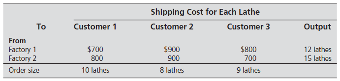
The Move-It Company has two plants producing forklift trucks that then are shipped to three distribution centers. The production costs are the same at the two plants, and the cost of shipping for each truck is shown for each combination of plant and distribution center: A total of 60 forklift trucks are produced and shipped per week. Each plant can produce and ship any amount up to a maximum of 50 trucks per week, so there is considerable flexibility on how to divide the total production between the two plants so as to reduce shipping costs. However, each distribution center must receive exactly 20 trucks per week. Management's objective is to determine how many forklift trucks should be produced at each plant, and then what the overall shipping pattern should be to minimize total shipping cost. (a) Formulate this problem as a transportation problem by constructing the appropriate parameter table. (b) Display the transportation problem on an Excel spreadsheet. C (c) Use the Excel Solver to obtain an optimal solution.
Redo Prob. 8.1-7 when any distribution center may receive any quantity between 10 and 30 forklift trucks per week in order to further reduce total shipping cost, provided only that the total shipped to all three distribution centers must still equal 60 trucks per week.

The Build-Em-Fast Company has agreed to supply its best customer with three widgets during each of the next 3 weeks, even though producing them will require some overtime work. The relevant production data are as follows: The cost per unit produced with overtime for each week is 100 more than for regular time. The cost of storage is $\$ 50$ per unit for each week it is stored. There is already an inventory of two wid-gets on hand currently, but the company does not want to retain any widgets in inventory after the 3 weeks. Management wants to know how many units should be produced in each week to minimize the total cost of meeting the delivery schedule. (a) Formulate this problem as a transportation problem by constructing the appropriate parameter table. C (b) Obtain an optimal solution.
The MJK Manufacturing Company must produce two products in sufficient quantity to meet contracted sales in each of the next three months. The two products share the same production facilities, and each unit of both products requires the same amount of production capacity. The available production and storage facilities are changing month by month, so the production capacities, unit production costs, and unit storage costs vary by month. Therefore, it may be worthwhile to overproduce one or both products in some months and store them until needed. For each of the three months, the second column of the following table gives the maximum number of units of the two products combined that can be produced on Regular Time (RT) and on Overtime (O). For each of the two products, the subsequent columns give (1) the number of units needed for the contracted sales, (2) the cost (in thousands of dollars) per unit produced on Regular Time, (3) the cost (in thousands of dollars) per unit produced on Overtime, and (4) the cost (in thousands of dollars) of storing each extra unit that is held over into the next month. In each case, the numbers for the two products are separated by a slash /, with the number for Product 1 on the left and the number for Product 2 on the right. The production manager wants a schedule developed for the number of units of each of the two products to be produced on Regular Time and (if Regular Time production capacity is used up) on Overtime in each of the three months. The objective is to minimize the total of the production and storage costs while meeting the contracted sales for each month. There is no initial inventory, and no final inventory is desired after the three months. (a) Formulate this problem as a transportation problem by constructing the appropriate parameter table. C (b) Obtain an optimal solution.

All The Dots Are Connected / It's Not Rocket Science
Transportation and assignment problems with r.
In the previous post “ Linear Programming with R ” we examined the approach to solve general linear programming problems with “Rglpk” and “lpSolve” packages. Today, let’s explore “lpSolve” package in depth with two specific problems of linear programming: transportation and assignment.
1. Transportation problem
Code & Output:
The solution is shown as lptrans$solution and the total cost is 20500 as lptrans$objval.
2. Assignment problem
Similarly, the solution and the total cost are shown as lpassign$solution and lpassign$objval respectively.

This article was really helpful, but I am facing issue while solving unbalanced transportation problem when there is excess demand. Could you please guide me on what has to be done in this case.

Hello sir, this article was really helpful. But, I am facing issue while solving unbalanced transportation problem when there is excess demand, it gives solution as no feasible solution. works perfectly fine for balanced and excess supply problems. Could you please guide me on why this issue is occurring and a possible solution for the same. Thank you.
Academia.edu no longer supports Internet Explorer.
To browse Academia.edu and the wider internet faster and more securely, please take a few seconds to upgrade your browser .
Enter the email address you signed up with and we'll email you a reset link.
- We're Hiring!
- Help Center

Transportation and Assignment Problems

Related Papers
sciepub.com SciEP
ام محمد لا للشات
manuel Carboni
Introducción En éste capítulo estudiaremos un modelo particular de problema de programación lineal, uno en el cual su resolución a través del método simplex es dispendioso, pero que debido a sus características especiales ha permitido desarrollar un método más práctico de solución. El modelo de transporte se define como una técnica que determina un programa de transporte de productos o mercancías desde unas fuentes hasta los diferentes destinos al menor costo posible. También estudiaremos el problema del transbordo en el que entre fuentes y destinos, existen estaciones intermedias. Por último estudiaremos el software WinQsb y el Invop.
Fatih Hamza
Evolutionary Computation
Zbigniew Michalewicz
Đào Thanh Duy
Cristian Choconta Diaz
International Journal of Engineering Sciences & Research Technology
Ijesrt Journal
The Transportation problem is a special class of Linear Programming Problem. It deals with shipping commodities from different sources to various destinations. The objective is to determine the shipping schedule that minimizes the total shipping cost while satisfying supply and demand limits. In general, the transportation model can be extended to areas other than the direct transportation of a commodity, including among others, inventory control, Engineering & Technology, Management sciences, Employment scheduling. In this paper, I have tried to reveal that the proposed direct methods namely NMD Method, Exponential Approach for finding optimal solution of a Transportation problem do not present optimal solution at all times.
IJERA Journal
Multi-objective transportation problem with fuzzy interval numbers are considered. The solution of linear MOTP is obtained by using non-linear membership functions. The optimal compromise solution obtained is compared with the solution got by using a linear membership function. Some numerical examples are presented to illustrate this.
RELATED PAPERS
Arthur Diax
Dama Academic Scholarly & Scientific Research Society
Journal of Applied Mathematics & Bioinformatics, Volume 6, No 2
Chowdhury Kibria
Juman Abdeen
Fabio Nobrega
subakir kholid
York Marcos Javier Díaz Wong
Applied Soft Computing
Ali Ebrahimnejad
Emerson Aguiar
basudeb datta
Mathematical Problems in Engineering
Hale Gonce Kocken
Proceedings of the 2010 International Conference on Industrial Engineering and Operations Management Dhaka, Bangladesh, January 9 – 10, 2010
AMALADAS JOHN RAJAN
IJCT Editor
IRJET Journal
International Journal of System Assurance Engineering and Management
Dr. P. Senthil Kumar (PSK), M.Sc., B.Ed., M.Phil., PGDCA., PGDAOR., Ph.D.,
Pakistan Journal of Biotechnology
Anand Jayakumar Arumugham
richmond opoku-sarkodie
AARF Publications Journals
Arcol Aries
Dimas Innocent
RELATED TOPICS
- We're Hiring!
- Help Center
- Find new research papers in:
- Health Sciences
- Earth Sciences
- Cognitive Science
- Mathematics
- Computer Science
- Academia ©2024
Balanced and Unbalanced Transportation Problems
The two categories of transportation problems are balanced and unbalanced transportation problems . As we all know, a transportation problem is a type of Linear Programming Problem (LPP) in which items are carried from a set of sources to a set of destinations based on the supply and demand of the sources and destinations, with the goal of minimizing the total transportation cost. It is also known as the Hitchcock problem.
Introduction to Balanced and Unbalanced Transportation Problems
Balanced transportation problem.
The problem is considered to be a balanced transportation problem when both supplies and demands are equal.
Unbalanced Transportation Problem
Unbalanced transportation problem is defined as a situation in which supply and demand are not equal. A dummy row or a dummy column is added to this type of problem, depending on the necessity, to make it a balanced problem. The problem can then be addressed in the same way as the balanced problem.
Methods of Solving Transportation Problems
There are three ways for determining the initial basic feasible solution. They are
1. NorthWest Corner Cell Method.
2. Vogel’s Approximation Method (VAM).
3. Least Call Cell Method.
The following is the basic framework of the balanced transportation problem:

The destinations D1, D2, D3, and D4 in the above table are where the products/goods will be transported from various sources O1, O2, O3, and O4. The supply from the source Oi is represented by S i . The demand for the destination Dj is d j . If a product is delivered from source Si to destination Dj, then the cost is called C ij .
Let us now explore the process of solving the balanced transportation problem using one of the ways known as the NorthWest Corner Method in this article.
Solving Balanced Transportation problem by Northwest Corner Method
Consider this scenario:

With three sources (O1, O2, and O3) and four destinations (D1, D2, D3, and D4), what is the best way to solve this problem? The supply for the sources O1, O2, and O3 are 300, 400, and 500, respectively. Demands for the destination D1, D2, D3, and D4 are 250, 350, 400, and 200, respectively.
The starting point for the North West Corner technique is (O1, D1), which is the table’s northwest corner. The cost of transportation is calculated for each value in the cell. As indicated in the diagram, compare the demand for column D1 with the supply from source O1 and assign a minimum of two to the cell (O1, D1).
Column D1’s demand has been met, hence the entire column will be canceled. The supply from the source O1 is still 300 – 250 = 50.

Analyze the northwest corner, i.e. (O1, D2), of the remaining table, excluding column D1, and assign the lowest among the supply for the appropriate column and rows. Because the supply from O1 is 50 and the demand for D2 is 350, allocate 50 to the cell (O1, D2).
Now, row O1 is canceled because the supply from row O1 has been completed. Hence, the demand for Column D2 has become 350 – 50 = 50.

The northwest corner cell in the remaining table is (O2, D2). The shortest supply from source O2 (400) and the demand for column D2 (300) is 300, thus putting 300 in the cell (O2, D2). Because the demand for column D2 has been met, the column can be deleted, and the remaining supply from source O2 is 400 – 300 = 100.

Again, find the northwest corner of the table, i.e. (O2, D3), and compare the O2 supply (i.e. 100) to the D2 demand (i.e. 400) and assign the smaller (i.e. 100) to the cell (O2, D2). Row O2 has been canceled because the supply from O2 has been completed. Column D3 has a leftover demand of 400 – 100 = 300.

Continuing in the same manner, the final cell values will be:

It should be observed that the demand for the relevant columns and rows is equal in the last remaining cell, which was cell (O3, D4). In this situation, the supply from O3 was 200, and the demand for D4 was 200, therefore this cell was assigned to it. Nothing was left for any row or column at the end.
To achieve the basic solution, multiply the allotted value by the respective cell value (i.e. the cost) and add them all together.
I.e., (250 × 3) + (50 × 1) + (300 × 6) + (100 × 5) + (300 × 3) + (200 × 2) = 4400.
Solving Unbalanced Transportation Problem
An unbalanced transportation problem is provided below. Because the sum of all the supplies, O1, O2, O3, and O4, does not equal the sum of all the demands, D1, D2, D3, D4, and D5, the situation is unbalanced.

The idea of a dummy row or dummy column will be applied in this type of scenario. Because the supply is more than the demand in this situation, a fake demand column will be inserted, with a demand of (total supply – total demand), i.e. 117 – 95 = 22, as seen in the image below. A fake supply row would have been introduced if demand was greater than supply.

Now this problem has been changed to a balanced transportation problem, and it can be addressed using any of the ways listed below to solve a balanced transportation problem, such as the northwest corner method mentioned earlier.
Frequently Asked Questions on Balanced and Unbalanced Transportation Problems
What is meant by balanced and unbalanced transportation problems.
The problem is referred to as a balanced transportation problem when both supplies and demands are equal. Unbalanced transportation is defined as a situation where supply and demand are not equal.
What is called a transportation problem?
The transportation problem is a type of Linear Programming Problem in which commodities are carried from a set of sources to a set of destinations while taking into account the supply and demand of the sources and destinations, respectively, in order to reduce the total cost of transportation.
What are the different methods to solve transportation problems?
The following are three approaches to solve the transportation issue:
- NorthWest Corner Cell Method.
- Least Call Cell Method.
- Vogel’s Approximation Method (VAM).
Leave a Comment Cancel reply
Your Mobile number and Email id will not be published. Required fields are marked *
Request OTP on Voice Call
Post My Comment
- Share Share
Register with BYJU'S & Download Free PDFs
Register with byju's & watch live videos.

IMAGES
VIDEO
COMMENTS
use the Stepping Stone method to nd an optimal solution of a transportation problem formulate special linear programming problems using the assignment model solve assignment problems with the Hungarian method. 4.2 Introduction In this unit we extend the theory of linear programming to two special linear programming problems, the Transportation ...
Prasad A Y, Dept of CSE, ACSCE, B'lore-74. Page 33. Module 4: Transportation Problem and Assignment problem. This means that programmer 1 is assigned programme C, programmer 2 is assigned programme A, and so on. The minimum time taken in developing the programmes is = 80 + 80 + 100 + 90 = 350 min.
7. Identify the relationship between assignment problems and transportation problems. 8. Formulate a spreadsheet model for an assignment problem from a description of the problem. 9. Do the same for some variants of assignment problems. 10. Give the name of an algorithm that can solve huge assignment problems that are well
44 9 · Transportation and Assignment Problems m ij i,j i P k:(i,k)∈Em ik −b i j P k:(j,k)∈Em jk −b j 0 c ij Figure 9.1: Representation of flow conservation constraints by a transportation problem We now construct a transportation problem as follows. For every vertex i ∈ V, we add a sink vertex with demand P km ik−b i. For every ...
154 Chapter5. Thetransportationproblemandtheassignmentproblem min z = (8 , 6 , 10 , 10 , 4 , 9) x11 x12 x13 x21 x22 x23 subjectto
This article provides a literature review of transportation problems and their solutions. The authors explore the various types of transportation problems and the available solutions that can be used to address them. ... Heuristic methods such as the greedy algorithm have been proposed to find approximate solutions to the assignment problem. â ...
An example based on the network view given in Figure TP-1 above is provided here: The Transportation Problem - Spreadsheet Formulation and Solution. Finally, at the next two links, we provide short descriptions of the assignment problem and the transshipment problem. The Assignment Problem: An Example. The Transshipment Problem: An Example
Transportation, Transshipment, and Assignment Problems Learning Objectives After completing this chapter, you should be able to: Describe the nature of transportation transshipment and assignment problems. Formulate a transportation problem as a linear programming model. Use the transportation method to solve problems with Excel.
Identify the relationship between assignment problems and transportation problems. Formulate a spreadsheet model for an assignment problem from a description of the problem. Do the same for some variants of assignment problems. Give the name of an algorithm that can solve huge assignment problems that are well beyond the scope of Solver.
Transportation and assignment problems are traditional examples of linear programming problems. Although these problems are solvable by using the techniques of Chapters 2-4 directly, the solution procedure is cumbersome; hence, we develop much more efficient algorithms for handling these problems. In the case of transportation problems, the ...
Transportation and assignment problems are traditional examples of linear programming problems. Although these problems are solvable by using the techniques of Chapters 2-4 directly, the solution procedure is cumbersome; hence, we develop much more efficient algorithms for handling these problems. In the case oftransportation problems, the ...
Transportation, Assignment, and ... timal solution to this balanced transportation problem is z 975, x 13 20, x 12 15, x 21 40, x 23 10, x 32 5, x 34 30, and x 35 5. Because x 35 5, 5 million kwh of plant 3 capacity will be unused (see Figure 2). A transportation problem is specified by the supply, the demand, and the shipping costs, so the ...
The Simplex Method for Transportation Problems. Illustrative Examples and a Note on Degeneracy. The Simplex Tableau Associated with a Transportation Tableau. The Assignment Problem: (Kuhn's) Hungarian Algorithm. Alternating Path Basis Algorithm for Assignment Problems. A Polynomial-Time Successive Shortest Path Approach for Assignment Problems
In the second part of this chapter, an assignment problem is discussed, which involves assigning people to tasks. The Hungarian method for solving assignment problems is presented. Various formulations for the problems are provided along with their solutions. All learning outcomes, solved examples, and questions are mapped with Bloom's ...
Transportation Problem •The transportation problem is solved in two phases: •Phase I -- Obtaining an initial feasible solution •Phase II -- Moving toward optimality •In Phase I, the Minimum-Cost Procedure can be used to establish an initial basic feasible solution without doing numerous iterations of the simplex method.
The problem is to allocate land use in each country so as to meet the world food requirement and minimize the total labor cost. (a) Formulate this problem as a transportation problem by constructing the appropriate parameter table. (b) Draw the network representation of this problem. C (c) Obtain an optimal solution.
Assignment or transportation 49. Prohibited routes (6-48) 50. ... Unbalanced assignment PROBLEM SOLUTIONS 1. St. Louis - Chicago = 250 Richmond - Chicago = 50 Richmond - Atalnta = 350 Chapter Six: Transportation, Transshipment, and Assignment Problems. 78 2. x13 = 2 x14 = 10 x22 = 9 x23 = 8 x31 = 10 x32 = 1 3. xA3 = 100 xB1 = 135 xB2 = 45 xC2 ...
Transportation and Assignment problems with R. In the previous post " Linear Programming with R " we examined the approach to solve general linear programming problems with "Rglpk" and "lpSolve" packages. Today, let's explore "lpSolve" package in depth with two specific problems of linear programming: transportation and ...
The Transportation problem is a special class of Linear Programming Problem. It deals with shipping commodities from different sources to various destinations.
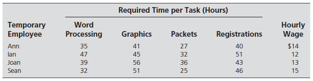
LP problems, the number of routes (or, in this case, assignments) must equal the number of sources or sites (in this case, workers) plus the number of destinations (in this case, jobs) minus one; is, Assignments = Workers + Jobs - 1; that is, Assignments = 6. - 1. We can see that for our problem, we have six nonempty cells.
Assignment model-Formulation, differences between Transportation problem and Assignment problem, Hungarian method-procedure and problems, Unbalanced Assignment problems. 10. ... Transportation Problem. Solution : The initial basic feasible solution using VAM is shown in table below. Initial Basic Feasible Solution Using VAM.
Unbalanced Transportation Problem. Example - 1: Check which types of Transportation Problem it is. Answer - 1: From the above, we have. Total Supply = 5 + 8 + 7 + 14 = 34. Total Demand = 7 + 9 + 18 = 34. Hence, Total Supply = Total Demand. Therefore, it is a Balanced Transportation Problem.
Unbalanced Transportation Problem. Unbalanced transportation problem is defined as a situation in which supply and demand are not equal. A dummy row or a dummy column is added to this type of problem, depending on the necessity, to make it a balanced problem. The problem can then be addressed in the same way as the balanced problem.