assignment 10.1 image labeling

ORIGINAL RESEARCH article

101 labeled brain images and a consistent human cortical labeling protocol.

• 1 Department of Psychiatry and Behavioral Science, Stony Brook University School of Medicine, Stony Brook, NY, USA
• 2 Department of Psychiatry, Columbia University, New York, NY, USA
• 3 Department of Speech, Language, and Hearing Sciences, Boston University, Boston, MA, USA
• 4 Center for Computational Neuroscience and Neural Technology, Boston University, Boston, MA, USA

We introduce the Mindboggle-101 dataset, the largest and most complete set of free, publicly accessible, manually labeled human brain images. To manually label the macroscopic anatomy in magnetic resonance images of 101 healthy participants, we created a new cortical labeling protocol that relies on robust anatomical landmarks and minimal manual edits after initialization with automated labels. The “Desikan–Killiany–Tourville” (DKT) protocol is intended to improve the ease, consistency, and accuracy of labeling human cortical areas. Given how difficult it is to label brains, the Mindboggle-101 dataset is intended to serve as brain atlases for use in labeling other brains, as a normative dataset to establish morphometric variation in a healthy population for comparison against clinical populations, and contribute to the development, training, testing, and evaluation of automated registration and labeling algorithms. To this end, we also introduce benchmarks for the evaluation of such algorithms by comparing our manual labels with labels automatically generated by probabilistic and multi-atlas registration-based approaches. All data and related software and updated information are available on the http://mindboggle.info/data website.

Introduction

Labeling the macroscopic anatomy of the human brain is instrumental in educating biologists and clinicians, visualizing biomedical data, localizing brain data for identification and comparison, and perhaps most importantly, subdividing brain data for analysis. Labeled anatomical subdivisions of the brain enable one to quantify and report brain imaging data within brain regions, which is routinely done for functional, diffusion, and structural magnetic resonance images (f/d/MRI) and positron emission tomography data.

Labeled regions are important in and of themselves for use in characterizing the morphometry of the brain. Brain morphology measures have been used as biological markers to characterize schizophrenia ( Cachia et al., 2008 ), early- vs. intermediate-onset bipolar disorder, as well as bipolar and unipolar depression ( Penttilä et al., 2009 ; Mangin et al., 2010 ; Kempton et al., 2011 ), and may someday aid clinicians in the diagnosis and prediction of treatment response for neuropsychiatric disorders. A biomarker of disease is defined by its ability to distinguish between clinical and control populations. Distinguishing among groups requires that the variation of a suitable measure within each group is separable from the variation between groups. This can only be accomplished by establishing “normative” data – data that allow accurate characterization of the usual variation within each group. Thus a significant hurdle to discovering better biomarkers for patient-specific psychiatric medicine is the lack of normative data to compare against. For this, we would need to carefully label the anatomy of many normal, healthy brains.

Another important application of labeled brain images is to train, test, and evaluate automated registration, segmentation, parcellation, and labeling algorithms. We conducted the world’s most extensive brain image registration evaluation studies ( Klein et al., 2009 , 2010b ), but this was made possible only because of the public availability of manually labeled brain image data. These studies guided our research and exposed the limitations of existing labeled data sets and labeling protocols. We need a greater number of consistently, comprehensively, and accurately labeled brain images to drive brain imaging methods development.

The human cerebral cortex is difficult to label due to the great anatomical variation in the cortical folds and difficulty in establishing consistent and accurate reference landmarks across the brain ( Ono et al., 1990 ; Petrides, 2011 ). Accurate definitions for landmarks and label boundaries is important because they underlie our assumptions of correspondence across brain image data. Although there is no ground truth to measure the accuracy of anatomical assignments, it is common to measure consistency across human labelers (e.g., Caviness et al., 1996 ) and variability across co-registered landmarks (e.g., Lohmann and von Cramon, 2000 ). There is a tradeoff between accuracy and efficiency, however. It takes a human operator 2–3 days to manually label a single brain image of 1 mm 3 resolution without any initial set of label candidates. Automated anatomical labeling can help to initialize the labeling and make the process more efficient, by registering the labels from a probabilistic atlas ( Bilder et al., 2008 ) or multiple individually labeled atlases ( Klein et al., 2005 ; Heckemann et al., 2006 ; Aljabar et al., 2009 ) to a brain image, or by using dedicated anatomical labeling software ( Fischl et al., 1999 ; Cointepas et al., 2001 ; Klein and Hirsch, 2005 ). Care must then be taken to reduce the bias of the human editor to the initialized set of automated labels. Hence an accurate, reproducible labeling protocol is crucial.

There are volume-based and surface-based cortical labeling protocols for delineating regions on either cross-referenced slices through an image volume or on inflated or flattened surface meshes. Examples of volume-based cortical labeling protocols include those developed at the Center for Morphometric Analysis at the Massachusetts General Hospital ( Caviness et al., 1996 ), the Montreal Neurological Institute ( Petrides, 2011 ), UCLA’s Laboratory of Neuro Imaging 1 ( Bilder et al., 2008 ), as well as the IOWA ( Crespo-Facorro et al., 2000 ), AAL ( Delcroix et al., 2002 ), and BrainCOLOR 2 ( Klein et al., 2010a ) protocols. The most popular surface-based human cortical labeling protocols are the Desikan–Killiany (DK; Desikan et al., 2006 ) and Destrieux protocols ( Destrieux et al., 2010 ) used by the FreeSurfer brain analysis software ( Dale et al., 1999 ; Fischl et al., 1999 , 2002 , 2001 ). It is very difficult to reconcile the differences between ( Bohland et al., 2009 ) or compare the accuracy of volume-based and surface-based labeling protocols or algorithms due to interpolation artifacts that are introduced when converting data from one space to another ( Klein et al., 2010a ). However, surface-based labeling protocols avoid the use of cutting planes that arbitrarily cut through a volume to connect landmarks, and anecdotal evidence suggests that they require less time to learn and to apply consistently.

We created a surface-based cortical labeling protocol to set a new standard of labeling accuracy and consistency for use by the scientific community, as well as to create the largest and most complete set of labeled brains ever released to the public, called the “Mindboggle-101” dataset because of its concurrent development and use with the Mindboggle automated labeling and shape analysis software. In this article we introduce this dataset of manually edited brain image labels applied to the T 1-weighted MR images of publicly available multi-modal data acquired from healthy individuals. We also introduce a benchmark for the evaluation of automated registration/segmentation/labeling methods by comparing the manual labels according to this “Desikan–Killiany–Tourville” (DKT) protocol with automatically generated labels. All data, software, and information related to this study will be available as a public resource on the http://mindboggle.info/data website under a Creative Commons license 3 .

Materials and Methods

We selected 101 T 1-weighted brain MR images that are: (1) publicly accessible with a non-restrictive license, (2) from healthy participants, (3) of high quality to ensure good surface reconstruction, and (4) part of a multi-modal acquisition ( T 2*-weighted, diffusion-weighted scans, etc.). Five subjects were scanned specifically for this dataset (MMRR-3T7T-2, Twins-2, and Afterthought-1). Scanner acquisition and demographic information are included as Supplementary Material and are also available on the http://mindboggle.info/data website. Table 1 lists the data sets that comprise the Mindboggle-101 data set. These include the 20 test–retest subjects from the “Open Access Series of Imaging Studies” data ( Marcus et al., 2007 ), the 21 test–retest subjects from the “Multi-Modal Reproducibility Resource” ( Landman et al., 2011 ), with two additional subjects run under the same protocol in 3T and 7T scanners, 20 subjects from the “Nathan Kline Institute Test–Retest” set, 22 subjects from the “Nathan Kline Institute/Rockland Sample”, the 12 “Human Language Network” subjects ( Morgan et al., 2009 ), the Colin Holmes 27 template ( Holmes et al., 1998 ), two identical twins (including author AK), and one brain imaging colleague.

Table 1 . Data sets comprising the Mindboggle-101 labeled data set .

We preprocessed and segmented T 1-weighted MRI volumes and constructed cortical surfaces using FreeSurfer’s standard recon-all image processing pipeline 4 ( Dale et al., 1999 ; Fischl et al., 1999 ). Since it has been demonstrated recently that FreeSurfer results can vary depending on software version, operating system, and hardware ( Gronenschild et al., 2012 ), every group of subjects was processed by FreeSurfer with the same computer setup. All images were run on Apple OSX 10.6 machines, except for two (Twins-2, run on Ubuntu 11.04), and all were run using FreeSurfer version 5.1.0, except for the OASIS-TRT-20, which were run using 5.0.0 (manual labeling was completed prior to the availability of v5.1.0). Following an initial pass, JT inspected segmentation and surface reconstructions for errors (manual edits to the gray–white tissue segmentation were required for a single subject: HLN-12-2). FreeSurfer then automatically labeled the cortical surface using its DK cortical parcellation atlas ([lh,rh].curvature.buckner40.filled.desikan_killiany.2007 06 20gcs for left and right hemispheres). Vertices along the cortical surface are assigned a given label based on local surface curvature and average convexity, prior label probabilities, and neighboring vertex labels ( S’egonne et al., 2004 ; Desikan et al., 2006 ). The region definitions of the labeling protocol represented by the DK atlas are described in Desikan et al. (2006) .

Desikan–Killiany–Tourville Labeling Protocol

The goal of this work was to create a large dataset of consistently and accurately labeled cortices. To do so we adopted a modification of the DK protocol ( Desikan et al., 2006 ). We modified the protocol for two reasons: (i) to make the region definitions as consistent and as unambiguous as possible, and (ii) to rely on region boundaries that are well suited to FreeSurfer’s classifier algorithm, such as sulcal fundi that are approximated by surface depth and curvature. This would make it easier for experienced raters to assess and edit automatically generated labels, and to minimize errors introduced by the automatic labeling algorithm. We also sought to retain major region divisions that are of interest to the neuroimaging community. In some cases, this necessitated the inclusion of anatomically variable sulci as boundary markers (such as subdivisions of the inferior frontal gyrus) or use of gyral crowns (such as the pericalarine cortex). Alternatively, common subdivisions of gyri that were not based on cortical surface curvature features (such as subdivisions of the cingulate gyrus and the middle frontal gyrus) were retained if the subdivision was wholly within the surface curvature features that defined the gyrus.

The DKT protocol has 31 cortical regions per hemisphere, one less than the DK protocol. We have also created a variant of the DKT protocol with 25 cortical regions per hemisphere to combine regions that are subdivisions of a larger gyral formation and whose divisions are not based on sulcal landmarks or are formed by sulci that are highly variable. The regions we combined include subdivisions of the cingulate gyrus, the middle frontal gyrus, and the inferior frontal gyrus. Since fewer regions means larger regions that lead to higher overlap measures when registering images to each other, note that comparisons should be made using the same labeling protocol. We refer to these two variants as the DKT31 and DKT25 cortical labeling protocols.

Figure 1 shows cortical regions in the DKT labeling protocol. We retained the coloring scheme and naming conventions of Desikan et al. (2006) for ease of comparison. The Appendix contains detailed definitions of the regions but we summarize modifications to the original DK protocol in Table 2 . Table 3 lists the names and abbreviations for the bounding sulci used by the DKT protocol; the locations of these sulci are demonstrated in Figure 2 . Three regions were eliminated from the original DK protocol: the frontal and temporal poles and the banks of the superior temporal sulcus. The poles were eliminated because their boundaries were comprised primarily of segments that “jumped” across gyri rather than along sulci. By redistributing these regions to surrounding gyri we have increased the portion of region boundaries that along similar curvature values, that is, along sulci and gyri rather than across them, which improves automatic labeling and the reliability of manual edits. The banks of the superior temporal sulcus region was eliminated because its anterior and posterior definitions were unclear and it spanned a major sulcus.

Figure 1. Regions in the DKT cortical labeling protocol . Cortical regions of interest included in the DKT protocol are displayed on the left hemisphere of the FreeSurfer “fsaverage” average brain template. Top : regions overlaid on lateral (left) and medial (right) views of the inflated cortical surface. The unlabeled area at the center of the medial view corresponds to non-cortical areas along the midline of the prosencephalon. Bottom : regions overlaid on lateral (upper left), medial (upper right), dorsal (lower left), and ventral (lower right) views of the pial surfaces. The surface was automatically labeled with the DKT40 classifier atlas then manually edited as needed. The “fsaverage” data are included in the FreeSurfer distribution in $FREESURFER_HOME/subjects/fsaverage and the DKT-labeled version is available at http://mindboggle.info/data .

Figure 2. Sulci in the DKT protocol . Sulci that form the region boundaries are drawn and labeled on the inflated “fsaverage” left hemisphere lateral (top left), medial (top right), and ventral (bottom) cortical surface. A map of surface curvature is indicated by the red-green colormap. Convex curvature corresponding to gyral crowns are shown in green; concave curvature corresponding to sulcal fundi are shown in red. The masked area at the center of the medial view corresponds to non-cortical areas along the midline of the prosencephalon. “*”, “**”, and “***” indicate the approximate locations of the transverse occipital sulcus, the temporal incisure, and the primary intermediate sulcus, respectively. These landmarks are not clearly distinguishable on the “fsaverage” inflated surface.

Table 2 . Cortical regions in the DKT labeling protocol .

Table 3 . Sulci included in the DKT labeling protocol and their abbreviations .

Additional, more minor, modifications took the form of establishing distinct sulcal boundaries when they approximated a boundary in the original protocol that was not clearly defined. For instance, the lateral boundary of the middle temporal gyrus anterior to the inferior frontal sulcus was defined explicitly as the lateral H-shaped orbital sulcus and the frontomarginal sulcus more anteriorly. Similarly, the boundary between the superior parietal and the lateral occipital regions was assigned to the medial segment of the transverse occipital sulcus. Other examples include establishing the rhinal sulcus and the temporal incisure as the lateral and anterior borders of the entorhinal cortex, and adding the first segment of the caudal superior temporal sulcus ( Petrides, 2011 ) as part of the posterior border of the supramarginal gyrus. Several popular atlases informed these modifications, including Ono et al. (1990) , Damasio (2005) , Duvernoy (1999) , and Mai et al. (2008) . The recent sulcus and gyrus atlas from Petrides (2011) proved particularly useful because of its exhaustive catalog of small but common sulci.

Label Editing Procedure

Greg Millington (GM) at Neuromorphometrics, Inc. 5 edited the initial labels under the supervision of JT to ensure adherence to the DKT protocol. The editing procedure is outlined in Figure 3 . GM relied on curvature maps overlaid on the native and inflated cortical (gray–white matter) surface and exterior cerebral (“pial”) surface to guide manual edits. JT inspected, and where necessary further edited, all manual edits. All manual edits were guided by the white matter, pial, and inflated surfaces, and the T1-weighted volume . While labeling was performed on the surface, we use topographical landmarks visible in the folded surface to infer label boundaries, so the volume remained the “ground truth” for evaluating anatomical decisions.

Figure 3. Label editing example . A typical manual edit is demonstrated. In the upper left, the pial surface of the right hemisphere is shown with labels generated from the DKT40 classifier atlas. Yellow arrowheads indicate a “double parallel” cingulate sulcus. The atlas failed to extend the rostral and caudal anterior cingulate regions dorso-rostrally to this sulcus, a common error when a parallel cingulate sulcus is present. To correct the error, the rater switches to the inflated surface view (upper right panel), and displays only the region outlines (lower right), which makes the cortical curvature map viewable. The rater then uses the curvature information to draw a line connecting vertices along the fundus of the parallel cingulate sulcus. Additional lines are drawn to subdivide the cingulate gyrus and the new regions are filled and labeled appropriately (bottom left panel). The yellow highlighted outline in the lower right panel indicates the last selected region (rostral anterior cingulate) and the light blue cursor mark within that region indicates the last selected surface vertex.

FreeSurfer’s DK classifier atlas assigned the initial labels for 54 of the brains in the Mindboggle-101 data set (OASIS-TRT-20, HLN-12, MMRR-21, and MMRR-3T7T-2). These were then manually edited by GM and JT to conform to the DKT protocol as described above. We selected the first 40 brains that we labeled (20 male, 20 female, 26 ± 7 years of age, from the MMRR-21, OASIS-TRT-20, and HLN-12 data) to train a new FreeSurfer cortical parcellation atlas representing the DKT protocol (see http://surfer.nmr.mgh.harvard.edu/fswiki/FsTutorial/GcaFormat ; S’egonne et al., 2004 ; Desikan et al., 2006 for details regarding the algorithm that generates the atlas and how it is implemented). The resulting “DKT40 classifier atlas” then automatically generated the initial set of cortical labels for the remaining 47 brains in the data set (see http://surfer.nmr.mgh.harvard.edu/fswiki/mris_ca_label ). To our knowledge, the DKT40 atlas was generated in the same manner as the DK atlas except for differences in the labeling protocol and training set.

Comparison of Manually Edited and Automated Labels

To set a benchmark for the evaluation of future automated registration, segmentation, and labeling methods, we computed the volume overlap between each manually labeled region in each of 42 subjects (NKI-RS-22 and NKI-TRT-20) and the corresponding automatically labeled region (in the same subject) generated by two automated labeling methods. The overlap measure was the Dice coefficient (equal to the intersection of the two regions divided by their average volume) and was computed after propagating the surface labels through the subject’s gray matter mask (using the command mri_aparc2aseg). For the first automated labeling method, we used FreeSurfer’s automated parcellation software once with the DK classifier atlas and separately with our DKT40 classifier atlas. The second method was a multi-atlas approach that registered multiple atlases to each subject. First we constructed two average FreeSurfer templates, one for the NKI-RS-22 group and the other for the NKI-TRT-20 group. We then used FreeSurfer’s surface-based registration algorithm to register all of the manually labeled NKI-RS-22 surfaces to each of the NKI-TRT-20 surfaces via the NKI-TRT-20 template, and likewise registered all of the manually labeled NKI-TRT-20 surfaces to each of the NKI-RS-22 surfaces via the NKI-RS-22 template. For each surface vertex in each subject, we then assigned a single label from the multiple registered labels by majority-vote rule, resulting in a set of maximum probability or majority-vote labels for each subject. The Python software for performing the multi-atlas labeling is available on the website: http://www.mindboggle.info/papers .

To demonstrate differences between the DK and DKT40 classifier atlases, we used both to label the Freesurfer “fsaverage” cortical surface template. Figure 4 shows mismatches between the automatically generated labels for the left hemisphere surface. In addition to differences associated with the removal of regions from the DK protocol (areas denoted by letters in Figure 4 ), several other areas of mismatch are notable (areas denoted by numbers). Mismatches in these areas are due to a number of sources, including changes in the boundary definitions of regions common to both protocols, high variability of some common region boundary landmarks, and variation in the interpretation of bounding landmarks. While there may be a primary cause of differences between the atlases, the mismatched areas shown in Figure 4 may be due to any combination of these factors. An additional source of variability contributing to the mismatch areas is the reliance on different training datasets for the construction of the two atlases. While there are several areas of mismatch, including large portions of some regions, the overall overlap of labels generated by the two classifier atlases was high: overall Dice overlap was 89% in the left hemisphere and 90% in the right hemisphere.

Figure 4. Comparison of DK and DKT40 classifier atlases . A comparison of the automatic labeling of the FreeSurfer “fsaverage” cortical surface by the DK and DKT40 atlases. Lateral ( upper left ), medial ( upper right ), ventral ( lower right ), and dorsal ( lower left ) views of the left hemisphere surface are shown. Regions in color overlaid atop the red-green surface (as in Figure 2 ) indicate areas that were labeled differently by the classifiers; where there are mismatches, the DKT40 labels are shown (with the same colors as in Figure 1 ). Areas denoted by letters mark the approximate location of regions in the DK protocol that were removed in the DKT protocol, including the banks of the superior temporal sulcus (b), frontal pole (f), and temporal pole (t). Additional, relatively large mismatched areas are denoted by numbers. Sources of mismatch between the protocols include: i, differences in region boundaries, particularly for the medial (1) and anterior (2) borders of pars orbitalis , the anterior border of the lateral orbitofrontal region (3), the lateral border of entorhinal cortex (4), and the anterior boundary of lateral orbital gyrus (5), and the posterior boundary of the superior parietal region (6); ii, variability of the bounding landmarks, particularly for the fundus of the parietooccipital sulcus (7) and the inferior frontal sulcus (8); iii, variation in the interpretation of landmarks, particularly for the cingulate sulcus (9), dorso-rostral portion of the circular sulcus (10), the rostral portion of superior frontal sulcus (11), the dorsal portion of the postcentral sulcus (12), the paracentral sulcus (13), and the posterior boundary of the medial and lateral orbitofrontal regions (14), and iv, variation in the training data set that was used to construct the classifier. The medial surface view was rotated from the parasagittal plane to expose the temporal pole.

Table 4 contains Dice overlap measures computed for each manually and automatically labeled cortical region, averaged across all of the 42 Nathan Kline subjects (NKI-RS-22 and NKI-TRT-20). The overlaps are higher than those computed in a prior study ( Klein et al., 2010b , Table 3 in Supplementary Material) which performed a single-atlas version of the multi-atlas labeling, confirming that it is better to use multiple atlases. Only the DKT and multi-atlas overlap values were generated using the same atlas brains following the DKT labeling protocol, so these values may be directly compared with one another (and not with the DK values). According to a Wilcoxon signed-rank test, the DKT mean overlap values are significantly greater than the multi-atlas mean overlap values ( p < 10 −10 ).

Table 4 . Overlap results of manually and automatically labeled cortical regions .

The Dice values are in general very high for the DKT auto/manual comparison (mean: 91 ± 6, range: 74–99). The Dice values are lower for regions that rely on anatomically variable sulci and when the region is bounded by discontinuous surface features. The pars orbitalis and pars triangularis , which had the lowest Dice coefficients, are affected by both factors. These relatively small regions are divided by the anterior horizontal ramus of the lateral sulcus. The length and location of this sulcus varies greatly with respect to nearby landmarks. Their anterior border is formed, in part, by another small, variable sulcus, the pretriangular sulcus. However, this sulcus rarely forms the entire anterior border of either region. Rather, the division between these regions and the more anterior middle frontal gyrus typically requires “jumps” across gyri. This makes reliable labeling of this region difficult for both an automatic algorithm and an experienced rater. A counter example is the insula (Dice > 98%) which is surrounded by a consistent, easily identified sulcus. Overlap measures are also biased in favor of larger regions.

In this article, we introduced the largest and most complete set of free, publicly available, manually labeled human brain images – 101 human cortices labeled according to a new surface-based cortical labeling protocol. These data are available 6 under a Creative Commons (attribution-non-commercial-sharealike 3.0) license (see text footnote 3). We compared the manual labels with labels generated by automated labeling methods to set benchmarks for the evaluation of automated registration/labeling methods.

Any automated labeling method could be used to initialize the labels for further editing by a human. We chose FreeSurfer for this study because it performs registration-based labeling well ( Klein et al., 2010b ), its classifier uses similar geometric properties such as local curvature that our DKT protocol follows, and because it offers a good interface for editing labels. And while the automated labeling algorithm turns the problem into one that is machine-assisted or semi-automatic, we use our manual labeling in turn to improve the automated labeling, in this study by creating a new classifier atlas. Our next step is to modify the current protocol to further improve the reliability and accuracy of both automatic and manual labeling. For instance, highly variable boundaries may be replaced or eliminated, resulting in the aggregation of existing labels (as in the DKT25 vs. DKT31 protocol). Alternatively, the experience of reviewing the cortical topography of such a large number of brains in a relatively short period of time has made apparent the existence of additional robust cortical features. For instance, the “temporo-limbic gyral passage” ( Petrides, 2011 ) is commonly observed in the basal temporal area. Adding this relatively small region to the protocol will make labeling this area of the brain more straightforward. We have also begun to use automatically extracted cortical features to refine these manual labels so that they follow stringent guidelines for curvature and depth, a difficult task for a human rater. Even without these aids, we were able to reduce the time required to label cortical regions to under 2 hours/brain of an experienced human rater’s time. Thus we are now able to label 10 or more brains in the time that one could be labeled fully manually, and with a similar level of accuracy.

Our original purpose for the Mindboggle-101 dataset was to create a publicly accessible online morphometry database to study anatomical variation, and for widespread use in training and testing automated algorithms. Other future goals include labeling more brain images from different demographic and clinical populations, creating more optimal average templates ( Avants et al., 2010 ) and probabilistic atlases based on these data, and incorporating what we learn from future labeling efforts into future versions of the labeling protocol (updates will be posted on http://mindboggle.info/data ).

Author Contributions

Arno Klein directed the labeling as part of the Mindboggle project, wrote and applied software for multi-atlas labeling, surface template construction, and evaluation of labels based on volume overlap measures, and wrote the manuscript. Jason Tourville created the cortical labeling protocol, supervised the manual labeling, performed the final labeling edits and approvals, constructed a new FreeSurfer atlas with some of the labeled data, and contributed to the writing of the manuscript.

Conflict of Interest Statement

The authors declare that the research was conducted in the absence of any commercial or financial relationships that could be construed as a potential conflict of interest.

Acknowledgments

We would like to thank Andrew Worth and Greg Millington of Neuromorphometrics, Inc., for their dedication to meticulous, consistent, and accurate manual labeling of brain image data. We are extremely grateful to Michael Milham, Bennett Landman, and Satrajit Ghosh for making multi-modal scans available for this project and for their shared interest in open data and open science. Arno Klein would also like to thank Deepanjana and Ellora for their continued support. This work was funded by the NIMH R01 grant MH084029 (“Mindboggling shape analysis and identification”). The OASIS project was funded by grants P50 AG05681, P01 AG03991, R01 AG021910, P50 MH071616, U24 RR021382, and R01 MH56584. The MMRR project was funded by NIH grants NCRR P41RR015241, 1R01NS056307, 1R21NS064534-01A109, and 1R03EB012461-01. The NKI project was funded primarily by R01 MH094639. The HLN project was funded by NIH grant EB000461.

Supplementary Material

The Supplementary Material for this article can be found online at http://www.frontiersin.org/Brain_Imaging_Methods/10.3389/fnins.2012.00171/abstract

• ^ http://www.loni.ucla.edu/Protocols/
• ^ http://www.braincolor.org
• ^ http://creativecommons.org/licenses/by-nc-sa/3.0/deed.en_US
• ^ http://surfer.nmr.mgh.harvard.edu/
• ^ http://www.neuromorphometrics.com
• ^ http://mindboggle.info/data/

Aljabar, P., Heckemann, R. A., Hammers, A., Hajnal, J. V., and Rueckert, D. (2009). Multi-atlas based segmentation of brain images: atlas selection and its effect on accuracy. Neuroimage 46, 726–738. doi:10.1016/j.neuroimage.2009.02.018

CrossRef Full Text

Avants, B. B., Yushkevich, P., Pluta, J., Minkoff, D., Korczykowski, M., Detre, J., et al. (2010). The optimal template effect in hippocampus studies of diseased populations. Neuroimage 49, 2457–2466.

Pubmed Abstract | Pubmed Full Text | CrossRef Full Text

Bilder, R. M., Toga, A. W., Mirza, M., Shattuck, D. W., Adisetiyo, V., Salamon, G., et al. (2008). Construction of a 3D probabilistic atlas of human cortical structures. Neuroimage 39, 1064–1080.

Bohland, J. W., Bokil, H., Mitra, P. P., and Allen, C. B. (2009). The brain atlas concordance problem: quantitative comparison of anatomical parcellations. PLoS ONE 4:e7200. doi:10.1371/journal.pone.0007200

Cachia, A., Paillère-Martinot, M.-L., Galinowski, A., Januel, D., de Beaurepaire, R., Bellivier, F., et al. (2008). Cortical folding abnormalities in schizophrenia patients with resistant auditory hallucinations. Neuroimage 39, 927–935. doi:10.1016/j.neuroimage.2007.08.049

Caviness, V. S., Meyer, J., Makris, N., and Kennedy, D. N. (1996). MRI-based topographic parcellation of human neocortex: an anatomically specified method with estimate of reliability. J. Cogn. Neurosci. 8, 566–587.

Cointepas, Y., Mangin, J.-F., Garnero, L., Poline, J.-B., and Benali, H. (2001). BrainVISA: software platform for visualization and analysis of multi-modality brain data. Hum. Brain Mapp. 13(Suppl.), :98.

Crespo-Facorro, B., Kim, J.-J., Andreasen, N. C., Spinks, R., O’Leary, D. S., Bockholt, H. J., et al. (2000). Cerebral cortex: a topographic segmentation method using magnetic resonance imaging. Psychiatry Res. 100, 97–126.

Dale, A. M., Fischl, B., and Sereno, M. I. (1999). Cortical surface-based analysis. I: segmentation and surface reconstruction. Neuroimage 9, 179–194.

Damasio, H. (2005). Human Brain Anatomy in Computerized Images , 2nd Edn. New York: Oxford University Press.

Delcroix, N., Tzourio-Mazoyer, N., Landeau, B., Papathanassiou, D., Crivello, F., Mazoyer, B., et al. (2002). Automated anatomical labeling of activations in SPM using a macroscopic anatomical parcellation of the MNI MRI single-subject brain. Neuroimage 15, 273–289.

Desikan, R. S., Segonne, F., Fischl, B., Quinn, B. T., Dickerson, B. C., Blacker, D., et al. (2006). An automated labeling system for subdividing the human cerebral cortex on MRI scans into gyral based regions of interest. Neuroimage 3, 968–980.

Destrieux, C., Fischl, B., Dale, A., and Halgren, E. (2010). Automatic parcellation of human cortical gyri and sulci using standard anatomical nomenclature. Neuroimage 53, 1–15. doi:10.1016/j.neuroimage.2010.06.010

Duvernoy, H. M. (1999). The Human Brain: Surface, Blood Supply, and Three Dimensional Anatomy . New York: Springer-Verlag Wien.

Fischl, B., Liu, A., and Dale, A. M. (2001). Automated manifold surgery: constructing geometrically accurate and topologically correct models of the human cerebral cortex. IEEE Trans. Med. Imaging 20, 70–80. doi:10.1109/42.906426

Fischl, B., Salat, D. H., Busa, E., Dale, A. M., Klaveness, S., Haselgrove, C., et al. (2002). Whole brain segmentation: neurotechnique automated labeling of neuroanatomical structures in the human brain. Neuron 33, 341–355.

Fischl, B., Sereno, M. I., and Dale, A. M. (1999). Cortical surface-based analysis II: Inflation, flattening, and a surface-based coordinate system. Neuroimage 9, 179–194.

Gronenschild, E. H. B. M., Habets, P., Jacobs, H. I. L., Mengelers, R., Rozendaal, N., van Os, J., et al. (2012). The effects of FreeSurfer Version, workstation type, and Macintosh Operating System Version on anatomical volume and cortical thickness measurements. PLoS ONE 7:e38234. doi:10.1371/journal.pone.0038234

Heckemann, R. A., Hajnal, J. V., Aljabar, P., Rueckert, D., and Hammers, A. (2006). Automatic anatomical brain {MRI} segmentation combining label propagation and decision fusion. Neuroimage 33, 115–126.

Holmes, C. J., Hoge, R., Collins, L., Woods, R., Toga, A. W., and Evans, A. C. (1998). Enhancement of MR images using registration for signal averaging. J. Comput. Assist. Tomogr. 22, 324–333.

Kempton, M. J., Salvador, Z., Munafò, M. R., Geddes, J. R., Simmons, A., Frangou, S., et al. (2011). Structural neuroimaging studies in major depressive disorder. Meta-analysis and comparison with bipolar disorder. Arch. Gen. Psychiatry 68, 675–690. doi:10.1001/archgenpsychiatry.2011.60

Klein, A., Andersson, J., Ardekani, B. A., Ashburner, J., Avants, B., Chiang, M.-C., et al. (2009). Evaluation of 14 nonlinear deformation algorithms applied to human brain MRI registration. Neuroimage 46, 786–802. doi:10.1016/j.neuroimage.2008.12.037

Klein, A., Dal Canton, T., Ghosh, S. S., Landman, B., Lee, J., and Worth, A. (2010a). Open labels: online feedback for a public resource of manually labeled brain images. 16th Annual Meeting for the Organization of Human Brain Mapping , Barcelona.

Klein, A., Ghosh, S. S., Avants, B., Yeo, B. T. T., Fischl, B., Ardekani, B., et al. (2010b). Evaluation of volume-based and surface-based brain image registration methods. Neuroimage 51, 214–220. doi:10.1016/j.neuroimage.2010.01.091

Klein, A., and Hirsch, J. (2005). Mindboggle: a scatterbrained approach to automate brain labeling. Neuroimage 24, 261–280. doi:10.1016/j.neuroimage.2004.09.016

Klein, A., Mensh, B., Ghosh, S., Tourville, J., and Hirsch, J. (2005). Mindboggle: automated brain labeling with multiple atlases. BMC Med. Imaging 5:7. doi:10.1186/1471-2342-5-7

Landman, B. A., Huang, A. J., Gifford, A., Vikram, D. S., Lim, I. A. L., Farrell, J. A. D., et al. (2011). Multi-parametric neuroimaging reproducibility: a 3-T resource study. Neuroimage 54, 2854–2866. doi:10.1016/j.neuroimage.2010.11.047

Lohmann, G., and von Cramon, D. Y. (2000). Automatic labelling of the human cortical surface using sulcal basins. Med. Image Anal. 4, 179–188.

Mai, J., Paxinos, G., and Voss, T. (2008). Atlas of the Human Brain . New York: Elsevier.

Mangin, J.-F., Jouvent, E., and Cachia, A. (2010). In-vivo measurement of cortical morphology: means and meanings. Curr. Opin. Neurol. 23, 359–367. doi:10.1097/WCO.0b013e32833a0afc

Marcus, D. S., Wang, T. H., Parker, J., Csernansky, J. G., Morris, J. C., and Buckner, R. L. (2007). Open access series of imaging studies (OASIS): cross-sectional MRI data in young, middle aged, nondemented, and demented older adults. J. Cogn. Neurosci. 19, 1498–1507.

Morgan, V. L., Mishra, A., Newton, A. T., Gore, J. C., and Ding, Z. (2009). Integrating functional and diffusion magnetic resonance imaging for analysis of structure–function relationship in the human language network. PLoS ONE 4:e6660. doi:10.1371/journal.pone.0006660

Ono, M., Kubik, S., and Abernathy, C. D. (1990). Atlas of the Cerebral Sulci . Stuttgart: Georg Thieme Verlag.

Penttilä, J., Cachia, A., Martinot, J.-L., Ringuenet, D., Wessa, M., Houenou, J., et al. (2009). Cortical folding difference between patients with early-onset and patients with intermediate-onset bipolar disorder. Bipolar Disord. 11, 361–370. doi:10.1111/j.1399-5618.2009.00683.x

Petrides, M. (2011). The Human Cerebral Cortex: An MRI Atlas of the Sulci and Gyri in MNI Stereotaxic Space . London: Academic Press.

S’egonne, F., Salat, D. H., Dale, A. M., Destrieux, C., Fischl, B., van der Kouwe, A., et al. (2004). Automatically parcellating the human cerebral cortex. Cereb. Cortex 14, 11–22.

Cortical Region Definitions

This labeling protocol is an adaptation of the DK cortical region definitions ( Desikan et al., 2006 ). Abbreviations below are for sulci (see Table 3 ) and anatomical terms of location:

A: anterior; P: posterior; V: ventral; D: dorsal; M: medial; L: lateral.

Temporal Lobe, medial aspect

Entorhinal cortex.

A: temporal incisure (rostral limit of cos ); P: posterior limit of the amygdala; D: medio-dorsal margin of the temporal lobe anteriorly, amygdala posteriorly; M: rhs ( cos ), or the cos if the rhs is not present.

Parahippocampal gyrus

A: posterior limit of the amygdala; P: posterior limit of the hippocampus; D: hippocampus; M: cos .

Temporal pole [removed]

The area included in the DK temporal pole has been redistributed to the superior, middle, and inferior temporal gyrus regions.

Fusiform gyrus

A: anterior limit of ots (anterior limit of cos ); P: first transverse sulcus posterior to the temporo-occipital notch (rostral limit of the superior parietal gyrus); M: cos ; L: ots .

Temporal Lobe, lateral aspect

Superior temporal gyrus.

A: anterior limit of the sts or a projection from the sts to the anterior limit of the temporal lobe; P: junction of phls (or its posterior projection) and caudal sts ( csts1 , 2 , or 3 ); M: The superior temporal gyrus includes the entire ventral bank of the ls with the exception of the transverse temporal gyrus, and therefore has a varying medial boundary. Listed from anterior to posterior they include, anterior to the temporo-frontal junction, the medial margin of the temporal lobe or the entorhinal cortex (posterior to the temporal incisures); crcs anterior to ftts ; the dorsolateral margin of the temporal lobe between anterior limits of ftts and hs ; hs anterior to the junction of hs and crcs ; lh anterior to phls ; phls ; L: sts .

Middle temporal gyrus

A: anterior limit of sts , P: aocs , M: sts anteriorly, posteriorly formed by csts3 ; L: its.

Inferior temporal gyrus

A: anterior limit of ifs ; P: aocs ; M: ots ; L: ifs .

Transverse temporal gyrus

A: anterior limit of ftts ; P: posterior limit of hs ; M: ftts ; L: hs ; between the anterior limits of ftts and hs , the lateral boundary is formed by the dorsolateral margin of the temporal lobe.

Banks of superior temporal sulcus [removed]

The area in the banks of the superior temporal sulcus in the DK protocol has been redistributed to the superior and middle temporal gyri.

Frontal Lobe

Superior frontal gyrus.

A: fms ; P: prcs (lateral surface); pcs (medial surface); M: cgs , sros anterior to anterior limit of cgs ; L: sfs .

Middle frontal gyrus

A: anterior limit of sfs ; P: prcs ; M: sfs ; L: ifs ; anterior to ifs , the ventro-lateral boundary is formed by fms and lhos .

The DK protocol divides the middle frontal gyrus into rostral and caudal subdivisions. The posterior limit of the ifs represents the approximate bounding landmark between the two regions. These regions remain in the DKT protocol; the division between the two was modified only if necessitated by changes in bounding sulci.

Inferior frontal gyrus, pars opercularis

A: aals ; P: prcs ; M: ifs ; L: crcs .

Inferior frontal gyrus, pars triangularis

A: prts ; P: aals ; M: ifs ; L: ahls ; if ahls does not extend anteriorly to prts , an anterior projection from ahls to prts completes the lateral boundary.

Inferior frontal gyrus, pars orbitalis

A: prts – if prts does not extend ventrally to the lhos , a ventral projection from prts to lhos completes the anterior boundary; P: posterior limit of orbitofrontal cortex; M: ahls – if ahls does not extend anteriorly to prts , an anterior projection from ahls to prts completes the lateral boundary; L: lhos .

Orbitofrontal, lateral division

A: fms ; P: posterior limit of orbitofrontal cortex; M: ofs ; L: lhos .

Orbitofrontal, medial division

A: fms ; P: posterior limit of orbitofrontal cortex; M: sros ; if sros merges with cgs , the medial/dorsal boundary is formed by cgs ; L: ofs .

Frontal pole [removed]

The area included in the DK frontal pole region has been redistributed to the superior frontal and orbitofrontal gyri.

Precentral gyrus

A: prcs ; P: cs ; M: dorsomedial hemispheric margin; L: crcs .

Paracentral lobule

A: pcs ; P: marginal ramus of cgs ; V: cgs ; D: dorsomedial hemispheric margin.

Parietal Lobe

Postcentral gyrus.

A: cs ; P: pocs ; M: dorsomedial hemispheric margin; L: crcs – if the lateral limit of pocs extends anterior to crcs , the posterior portion of the lateral/ventral boundary is formed by the lateral sulcus.

Supramarginal gyrus

A: pocs ; P: the supramarginal gyrus is formed by sulci demarcating the cortical convolution surrounding the pals – posteriorly, this is typically formed by pis medially, and csts1 laterally; M: itps ; L: ls anterior to phls , phls posteriorly.

Superior parietal

A: pocs ; P: tranverse sulcus lying immediately posterior to the pos – this is described as the tocs , medial segment, by Petrides (2011) ; M: dorsomedial hemispheric margin; L: itps .

Inferior parietal

A: csts1 ; P: junction of locs and itps ; M: itps ; L: locs anteriorly, tocs , lateral segment, posteriorly.

A: marginal ramus of cgs dorsally, sbps ventrally; P: pos ; V: ccs ; D: dorsomedial hemispheric margin.

Occipital Lobe

Lingual gyrus.

A: posterior limit of the hippocampus; P: posterior limit of ccs ; M: ccs anteriorly, medial limit of the ventral bank of ccs posterior to the junction of pos and ccs ; L: cos .

Pericalcarine cortex

A: junction of ccs and pos ; P: posterior limit of ccs ; D: dorsomedial margin of ccs ; V: ventromedial margin of ccs .

Cuneus cortex

A: pos ; P: posterior limit of ccs ; V: dorsomedial margin of ccs ; D: dorsomedial hemispheric margin.

Lateral occipital cortex

A: temporo-occipital notch laterally, aocs more medially, tocs , medial segment, medial to itps ; P: posterior limit of the occipital lobe; M: locs anteriorly; tocs , lateral segment, posteriorly; L: ots anteriorly; cos posterior to the transverse sulcus that marks the posterior limit of the fusiform gyrus; posterior to the posterior limit of cos , the lateral occipital cortex includes occipital cortex in its entirety.

Cingulate cortex

A/D: cgs ; in the event of a “double parallel cingulate,” (e.g., Ono et al., 1990 ), the A/D boundary of the cingulate is formed by the more anterior-dorsal branch of the cgs ; P: sbps ; V: The cingulate gyrus is formed by the cortical convolution that lies dorsal to the corpus callosum, extending antero-ventrally around the cc genu and postero-ventrally around the cc splenium. Dorsal to the corpus callosum, the ventral boundary is formed by the cas . In the subgenual area, it is formed by the cgs and in the subsplenial area by the ccs . The DK atlas subdivides the cingulate gyrus into the subdivisions listed below from anterior to posterior locations with their bounding landmarks. These regions were left in the current protocol. Divisions between these regions were modified only if necessitated by changes in bounding sulci.

Rostral anterior

A: cgs ; P: cc genu.

Caudal anterior

A: cc genu; P: mammillary bodies.

A: mammillary bodies; P: junction of the sbps and cgs (approximately).

A: junction of the sbps and cgs (approximately); P: sbps .

Keywords: human brain, cerebral cortex, MRI, anatomy, parcellation, labeling, segmentation

Citation: Klein A and Tourville J (2012) 101 labeled brain images and a consistent human cortical labeling protocol. Front. Neurosci. 6 :171. doi: 10.3389/fnins.2012.00171

Received: 28 July 2012; Paper pending published: 17 September 2012; Accepted: 14 November 2012; Published online: 05 December 2012.

Reviewed by:

Copyright: © 2012 Klein and Tourville. This is an open-access article distributed under the terms of the Creative Commons Attribution License , which permits use, distribution and reproduction in other forums, provided the original authors and source are credited and subject to any copyright notices concerning any third-party graphics etc.

*Correspondence: Arno Klein, Department of Psychiatry and Behavioral Science, Stony Brook University School of Medicine, HSC T-10, Stony Brook, NY 11794-8101, USA. e-mail: arno@binarybottle.com

† Arno Klein and Jason Tourville have contributed equally to this work.

Disclaimer: All claims expressed in this article are solely those of the authors and do not necessarily represent those of their affiliated organizations, or those of the publisher, the editors and the reviewers. Any product that may be evaluated in this article or claim that may be made by its manufacturer is not guaranteed or endorsed by the publisher.

• Docs Datagen's knowledge base
• SDK Quickstart Dagen's knowledge base
• API Datagen's knowledge base

• Smart-office
• Fitness applications
• Facial applications
• Facial recognition
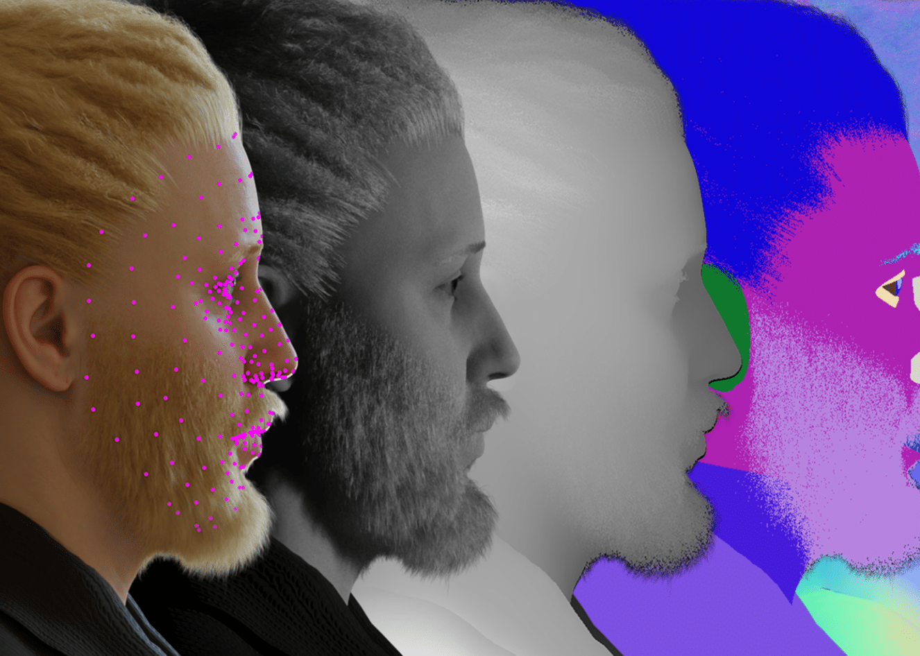
• Face and hair segmentation
• Eye gaze estimation
• Documentation
• SDK Quickstart
• Code templates
• Benchmark reports
• Survey reports
• Synthetic data
• Image annotation
• Image datasets
• Computer vision
• Training data

Home » Image Labeling in Computer Vision: A Practical Guide

Image Labeling in Computer Vision: A Practical Guide

What is Image Labeling?

Image labeling is a type of data labeling that focuses on identifying and tagging specific details in an image.

In computer vision, data labeling involves adding tags to raw data such as images and videos. Each tag represents an object class associated with the data. Supervised machine learning models employ labels when learning to identify a specific object class in unclassified data. It helps these models associate meaning to data, which can help train a model. 

Image annotation is used to create datasets for computer vision models, which are split into training sets, used to initially train the model, and test/validation sets used to evaluate model performance. Data scientists use the dataset to train and evaluate their model, and then the model can automatically assign labels to unseen, unlabelled data.

In This Article

Why is Image Labeling Important for AI and Machine Learning?

Image labeling is a key component of developing supervised models with computer vision capabilities. It helps train machine learning models to label entire images, or identify classes of objects within an image. Here are several ways in which image labeling helps:

• Developing functional artificial intelligence (AI) models— image labeling tools and techniques help highlight or capture specific objects in an image. These labels make images readable by machines, and highlighted images often serve as training data sets for AI and machine learning models. 
• Improving computer vision —image labeling and annotation helps improve computer vision accuracy by enabling object recognition. Training AI and machine learning with labels helps these models identify patterns until they can recognize objects on their own.

Types of Computer Vision Image Labeling

Image labeling is a core function in computer vision algorithms. Here are a few ways computer vision systems label images. The end goal of machine learning algorithms is to achieve labeling automatically, but in order to train a model, it will need a large dataset of pre-labelled images.

Image Classification

Image classification algorithms receive images as an input and are able to automatically classify them into one of several labels (also known as classes). For example, an algorithm might be able to classify images of vehicles into labels like “car”, “train”, or “ship”. 

In some cases, the same image might have multiple labels. In the example above, this could occur if the same image contains several types of vehicles.

Creating training datasets

To create a training dataset for image classification, it is necessary to manually review images and annotate them with labels used by the algorithm. For example, a training dataset for transportation images will include a large number of images containing vehicles, and a person would be responsible for looking at each image and applying the appropriate label—“car”, “train”, “ship”, etc. Alternatively, it is possible to generate such a dataset using synthetic data techniques.

• Semantic Segmentation

In semantic image segmentation, a computer vision algorithm is tasked with separating objects in an image from the background or other objects. This typically involves creating a pixel map of the image, with each pixel containing a value of 1 if it belongs to the relevant object, or 0 if it does not.

If there are multiple objects in the same image, typically the approach is to create multiple pixel objects, one for each object, and concatenate them channel-wise. 

To create a training dataset for a semantic segmentation dataset, it is necessary to manually review images and draw the boundaries of relevant objects. This creates a human-validated pixel map, which can be used to train the model. Alternatively, it is possible to generate pixel maps by creating synthetic images in which object boundaries are already known.

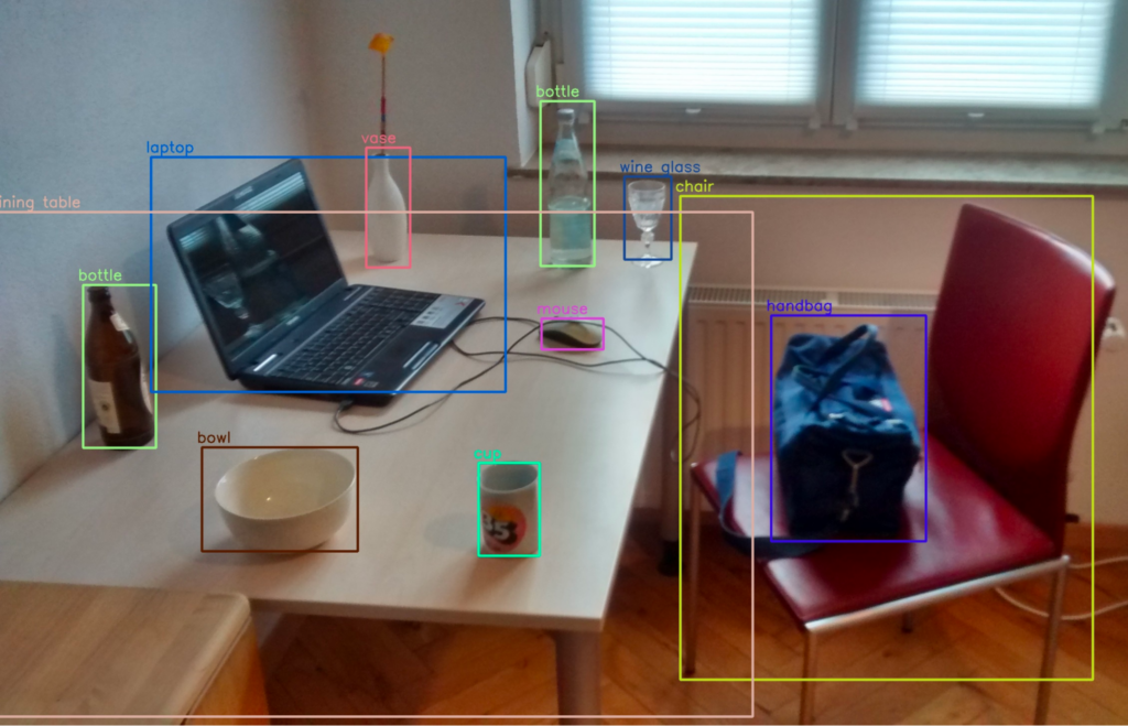
Object Detection

An object detection algorithm is tasked with detecting an object in an image and its location in the image frame. The location of objects are typically defined using bounding boxes. A bounding box is the smallest rectangle that contains the entire object in the image. 

Technically, a bounding box is a set of four coordinates, assigned to a label which specifies the class of the object. The coordinates of bounding boxes and their labels are typically stored in a JSON file, using a dictionary format. The image number or ID is the key in the dictionary file. 

The following image shows a scene with multiple bounding boxes denoting different objects.

Pose Estimation

A pose estimation algorithm is tasked with identifying the post of humans in an image. It attempts to detect several key points in the human body, and use them to understand the pose of the person in an image (for example, standing, sitting, or lying down).

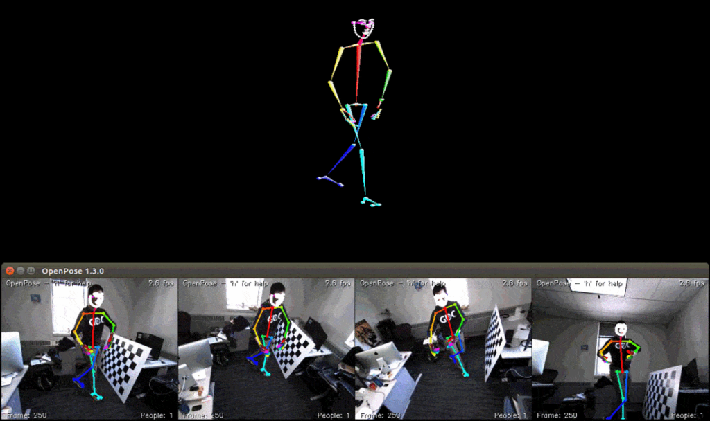
A training dataset for pose estimation contains images of people, with manual annotations indicating the key points of bodies appearing in the image. Technically, pose annotations are coordinates that are matched to labels, indicating which point in the human body is indicated (for example, the left hip). It is also possible to generate synthetic images of humans, in which the coordinates of key body points are already known.

Generate Synthetic Data with Our New Free Trial. Start now!

Methods of image labeling, manual image annotations.

A common way to label images is manual annotation. This is the process of manually defining labels for an entire image, or drawing regions in an image and adding textual descriptions of each region. 

Image annotation sets a standard, which a computer vision algorithm tries to learn from. This means that any errors in labeling will be adopted by the algorithm, reducing its accuracy. This means that accurate image labeling is a critical task in training neural networks. 

Manual annotation is typically assisted by tools that allow operators to rotate through a large number of images, draw regions on an image and assign labels, and save this data to a standardized format that can be used for data training.

Manual image annotation presents several challenges:

• Labels can be inconsistent if there are multiple annotators, and to resolve this, images need to be labeled several times with majority voting.
• Manual labeling is time consuming. Annotators must be meticulously trained and the process requires many iterations. This can delay time to market for computer vision projects.
• Manual labeling is costly and is difficult to scale to achieve large datasets.

Semi-Automated Image Annotations

Manual image annotation is a time-consuming task, and for some computer vision algorithms, can be difficult for humans to achieve. For example, some algorithms require creating pixel maps indicating the exact boundary of multiple objects in an image. 

Automated annotation tools can assist manual annotators, by attempting to detect object boundaries in an image, and providing a starting point for the annotator. Automated annotation algorithms are not completely accurate, but they can save time for human annotators by providing at least a partial map of objects in the image. 

Synthetic Image Labeling

Synthetic image labeling is an accurate and cost-effective technique which can replace manual annotations. It involves automatically generating images that are similar to real data, in accordance with criteria set by the operator. For example, it is possible to create a synthetic database of real-life objects or human faces, which are similar but not identical to real objects.

The main advantage of synthetic images is that labels are known in advance—for example, the operator automatically generates images containing tables and chairs. In this case, the algorithm generating the images can automatically provide the bounding boxes of the tables and chairs in each image.

There are three common approaches to generating synthetic images:

• Variational Autoencoders (VAE) —these are algorithms that start from existing data, create a new data distribution, and map it back to the original space using an encoder-decoder method.
• Generative Adversarial Networks (GAN) —these are models that pit two neural networks against each other. One neural network attempts to create fake images, while the other tries to distinguish real and fake images. Over time, the system becomes able to generate photorealistic images that are difficult to distinguish from real ones.
• Neural Radiance Fields (NeRF) —this model takes a series of images describing a 3D scene and automatically renders novel, additional viewpoints from the same scene. It works by computing a five-dimensional ray function to generate each voxel of the target image.

Learn More About Image Annotation

• Image Annotation Tools
• Image Segmentation
• Image Annotation
• Image Labeling

Get our free eBook

How to use synthetic data in 6 easy steps

The State of Facial Recognition Today

Procedural Humans for Computer Vision

Synthetic Data: Simulation & Visual Effects at Scale

We care about your data, and we would love to use cookies to make your experience better. our privacy policy ..

Label the Major Structures of the Brain

A = parietal labe | B = gyrus of the cerebrum | C = corpus callosum | D = frontal lobe E = thalamus | F = hypothalamus | G = pituitary gland | H = midbrain J = pons | K = medulla oblongata | L = cerebellum | M = transverse fissure | N = occipital lobe

Image Labeling by Assignment

• Published: 12 January 2017
• Volume 58 , pages 211–238, ( 2017 )

Cite this article

• Freddie Åström 1 ,
• Stefania Petra 2 ,
• Bernhard Schmitzer 3 &
• Christoph Schnörr   ORCID: orcid.org/0000-0002-8999-2338 4  

991 Accesses

44 Citations

1 Altmetric

Explore all metrics

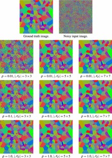
We introduce a novel geometric approach to the image labeling problem. Abstracting from specific labeling applications, a general objective function is defined on a manifold of stochastic matrices, whose elements assign prior data that are given in any metric space, to observed image measurements. The corresponding Riemannian gradient flow entails a set of replicator equations, one for each data point, that are spatially coupled by geometric averaging on the manifold. Starting from uniform assignments at the barycenter as natural initialization, the flow terminates at some global maximum, each of which corresponds to an image labeling that uniquely assigns the prior data. Our geometric variational approach constitutes a smooth non-convex inner approximation of the general image labeling problem, implemented with sparse interior-point numerics in terms of parallel multiplicative updates that converge efficiently.

This is a preview of subscription content, log in via an institution to check access.

Access this article

Price includes VAT (Russian Federation)

Instant access to the full article PDF.

Rent this article via DeepDyve

Institutional subscriptions

Similar content being viewed by others

Geometric Image Labeling with Global Convex Labeling Constraints

A Variational Perspective on the Assignment Flow

Unsupervised Assignment Flow: Label Learning on Feature Manifolds by Spatially Regularized Geometric Assignment

For locations i close to the boundary of the image domain where patch supports \({\mathscr {N}}_{p}(i)\) shrink, the definition of the vector \(w^{p}\) has to be adapted accordingly.

Amari, S.I., Nagaoka, H.: Methods of Information Geometry. American Mathematical Society, Oxford University Press, Oxford (2000)

MATH   Google Scholar  

Aujol, J.F., Gilboa, G., Chan, T., Osher, S.: Structure-texture image decomposition-modeling, algorithms, and parameter selection. Int. J. Comput. Vis. 67 (1), 111–136 (2006)

Article   MATH   Google Scholar  

Ball, K.: An elementary introduction to modern convex geometry. In: Levy, S. (ed.) Flavors of Geometry, MSRI Publ., vol. 31, pp. 1–58. Cambridge University Press (1997)

Bayer, D., Lagarias, J.: The nonlinear geometry of linear programming. I. Affine and projective scaling trajectories. Trans. Am. Math. Soc. 314 (2), 499–526 (1989)

MathSciNet   MATH   Google Scholar  

Bayer, D., Lagarias, J.: The nonlinear geometry of linear programming. II. Legendre transform coordinates and central trajectories. Trans. Am. Math. Soc. 314 (2), 527–581 (1989)

Bishop, C.: Pattern Recognition and Machine Learning. Springer, Berlin (2006)

Bomze, I., Budinich, M., Pelillo, M., Rossi, C.: Annealed replication: a new heuristic for the maximum clique problem. Discr. Appl. Math. 121 , 27–49 (2002)

Article   MathSciNet   MATH   Google Scholar  

Bomze, I.M.: Regularity versus degeneracy in dynamics, games, and optimization: a unified approach to different aspects. SIAM Rev. 44 (3), 394–414 (2002)

Buades, A., Coll, B., Morel, J.: A review of image denoising algorithms, with a new one. SIAM Multiscale Model. Simul. 4 (2), 490–530 (2005)

Buades, A., Coll, B., Morel, J.M.: Neighborhood filters and PDEs. Numer. Math. 105 , 1–34 (2006)

Cabrales, A., Sobel, J.: On the limit points of discrete selection dynamics. J. Econ. Theory 57 , 407–419 (1992)

Čencov, N.: Statistical Decision Rules and Optimal Inference. American Mathematical Society, Providence (1982)

Google Scholar  

Chambolle, A., Cremers, D., Pock, T.: A convex approach to minimal partitions. SIAM J. Imaging Sci. 5 (4), 1113–1158 (2012)

Chan, T., Esedoglu, S., Nikolova, M.: Algorithms for Finding Global Minimizers of Image Segmentation and Denoising Models. SIAM J. Appl. Math. 66 (5), 1632–1648 (2006)

Hérault, L., Horaud, R.: Figure-ground discrimination: a combinatorial optimization approach. IEEE Trans. Pattern Anal. Mach. Intell. 15 (9), 899–914 (1993)

Article   Google Scholar  

Heskes, T.: Convexity arguments for efficient minimization of the Bethe and Kikuchi free energies. J. Artif. Intell. Res. 26 , 153–190 (2006)

Hofbauer, J., Siegmund, K.: Evolutionary game dynamics. Bull. Am. Math. Soc. 40 (4), 479–519 (2003)

Hofman, T., Buhmann, J.: Pairwise data clustering by deterministic annealing. IEEE Trans. Pattern Anal. Mach. Intell. 19 (1), 1–14 (1997)

Horst, R., Tuy, H.: Global Optimization: Deterministic Approaches, 3rd edn. Springer, Berlin (1996)

Book   MATH   Google Scholar  

Hummel, R., Zucker, S.: On the foundations of the relaxation labeling processes. IEEE Trans. Pattern Anal. Mach. Intell. 5 (3), 267–287 (1983)

Jost, J.: Riemannian Geometry and Geometric Analysis, 4th edn. Springer, Berlin (2005)

Kappes, J., Andres, B., Hamprecht, F., Schnörr, C., Nowozin, S., Batra, D., Kim, S., Kausler, B., Kröger, T., Lellmann, J., Komodakis, N., Savchynskyy, B., Rother, C.: A comparative study of modern inference techniques for structured discrete energy minimization problems. Int. J. Comput. Vis. 115 (2), 155–184 (2015)

Article   MathSciNet   Google Scholar  

Kappes, J., Savchynskyy, B., Schnörr, C.: A bundle approach to efficient MAP-inference by Lagrangian relaxation. In: Proc. CVPR (2012)

Kappes, J., Schnörr, C.: MAP-inference for highly-connected graphs with DC-programming. In: Pattern Recognition—30th DAGM Symposium, LNCS, vol. 5096, pp. 1–10. Springer (2008)

Karcher, H.: Riemannian center of mass and mollifier smoothing. Commun. Pure Appl. Math. 30 , 509–541 (1977)

Karcher, H.: Riemannian center of mass and so called karcher mean. arxiv:1407.2087 (2014)

Kass, R.: The geometry of asymptotic inference. Stat. Sci. 4 (3), 188–234 (1989)

Kolmogorov, V.: Convergent tree-reweighted message passing for energy minimization. IEEE Trans. Pattern Anal. Mach. Intell. 28 (10), 1568–1583 (2006)

Kolmogorov, V., Zabih, R.: What energy functions can be minimized via graph cuts? IEEE Trans. Pattern Anal. Mach. Intell. 26 (2), 147–159 (2004)

Ledoux, M.: The Concentration of Measure Phenomenon. American Mathematical Society, Providence (2001)

Lellmann, J., Lenzen, F., Schnörr, C.: Optimality bounds for a variational relaxation of the image partitioning problem. J. Math. Imaging Vis. 47 (3), 239–257 (2013)

Lellmann, J., Schnörr, C.: Continuous multiclass labeling approaches and algorithms. SIAM J. Imaging Sci. 4 (4), 1049–1096 (2011)

Losert, V., Alin, E.: Dynamics of games and genes: discrete versus continuous time. J. Math. Biol. 17 (2), 241–251 (1983)

Luce, R.: Individual Choice Behavior: A Theoretical Analysis. Wiley, New York (1959)

Milanfar, P.: A tour of modern image filtering. IEEE Signal Process. Mag. 30 (1), 106–128 (2013)

Milanfar, P.: Symmetrizing smoothing filters. SIAM J. Imaging Sci. 6 (1), 263–284 (2013)

Montúfar, G., Rauh, J., Ay, N.: On the fisher metric of conditional probability polytopes. Entropy 16 (6), 3207–3233 (2014)

Nesterov, Y., Todd, M.: On the riemannian geometry defined by self-concordant barriers and interior-point methods. Found. Comput. Math. 2 , 333–361 (2002)

Orland, H.: Mean-field theory for optimization problems. J. Phys. Lett. 46 (17), 763–770 (1985)

Pavan, M., Pelillo, M.: Dominant sets and pairwise clustering. IEEE Trans. Pattern Anal. Mach. Intell. 29 (1), 167–172 (2007)

Pelillo, M.: The dynamics of nonlinear relaxation labeling processes. J. Math. Imaging Vis. 7 , 309–323 (1997)

Pelillo, M.: Replicator equations, maximal cliques, and graph isomorphism. Neural Comput. 11 (8), 1933–1955 (1999)

Rosenfeld, A., Hummel, R., Zucker, S.: Scene labeling by relaxation operations. IEEE Trans. Syst. Man Cybern. 6 , 420–433 (1976)

Singer, A., Shkolnisky, Y., Nadler, B.: Diffusion interpretation of non-local neighborhood filters for signal denoising. SIAM J. Imaging Sci. 2 (1), 118–139 (2009)

Sutton, R., Barto, A.: Reinforcement Learning, 2nd edn. MIT Press, Cambridge (1999)

Swoboda, P., Shekhovtsov, A., Kappes, J., Schnörr, C., Savchynskyy, B.: Partial optimality by pruning for MAP-inference with general graphical models. IEEE Trans. Patt. Anal. Mach. Intell. 38 (7), 1370–1382 (2016)

Wainwright, M., Jordan, M.: Graphical models, exponential families, and variational inference. Found. Trends Mach. Learn. 1 (1–2), 1–305 (2008)

Weickert, J.: Anisotropic Diffusion in Image Processing. B.G Teubner, Leipzig (1998)

Werner, T.: A linear programming approach to max-sum problem: a review. IEEE Trans. Pattern Anal. Mach. Intell. 29 (7), 1165–1179 (2007)

Yedidia, J., Freeman, W., Weiss, Y.: Constructing free-energy approximations and generalized belief propagation algorithms. IEEE Trans. Inf. Theory 51 (7), 2282–2312 (2005)

Download references

Acknowledgements

Support by the German Research Foundation (DFG) was gratefully acknowledged, Grant GRK 1653.

Author information

Authors and affiliations.

Heidelberg Collaboratory for Image Processing, Heidelberg University, Heidelberg, Germany

Freddie Åström

Mathematical Imaging Group, Heidelberg University, Heidelberg, Germany

Stefania Petra

CEREMADE, University Paris-Dauphine, Paris, France

Bernhard Schmitzer

Image and Pattern Analysis Group, Heidelberg University, Heidelberg, Germany

Christoph Schnörr

You can also search for this author in PubMed   Google Scholar

Corresponding author

Correspondence to Christoph Schnörr .

Appendix 1: Basic Notation

For \(n \in {\mathbb {N}}\) , we set \([n] = \{1,2,\ldots ,n\}\) . \({\mathbbm {1}}= (1,1,\ldots ,1)^{\top }\) denotes the vector with all components equal to 1, whose dimension can either be inferred from the context or is indicated by a subscript, e.g.,  \({\mathbbm {1}}_{n}\) . Vectors \(v^{1}, v^{2},\ldots \) are indexed by lowercase letters and superscripts, whereas subscripts \(v_{i},\, i \in [n]\) , index vector components. \(e^{1},\ldots ,e^{n}\) denotes the canonical orthonormal basis of \(\mathbb {R}^{n}\) .

We assume data to be indexed by a graph \({\mathscr {G}}=({\mathscr {V}},{\mathscr {E}})\) with nodes \(i \in {\mathscr {V}}=[m]\) and associated locations \(x^{i} \in \mathbb {R}^{d}\) , and with edges \({\mathscr {E}}\) . A regular grid graph and \(d=2\) is the canonical example. But \({\mathscr {G}}\) may also be irregular due to some preprocessing like forming super-pixels, for instance, or correspond to 3D images or videos ( \(d=3\) ). For simplicity, we call i location although this actually is \(x^{i}\) .

If \(A \in \mathbb {R}^{m \times n}\) , then the row and column vectors are denoted by \(A_{i} \in \mathbb {R}^{n},\, i \in [m]\) and \(A^{j} \in \mathbb {R}^{m},\, j \in [n]\) , respectively, and the entries by \(A_{ij}\) . This notation of row vectors \(A_{i}\) is the only exception from our rule of indexing vectors stated above.

The componentwise application of functions \(f :\mathbb {R}\rightarrow \mathbb {R}\) to a vector is simply denoted by f ( v ), e.g., 

Likewise, binary relations between vectors apply componentwise, e.g., \(u \ge v \;\Leftrightarrow \; u_{i} \ge v_{i},\; i \in [n]\) , and binary componentwise operations are simply written in terms of the vectors. For example,

where the latter operation is only applied to strictly positive vectors \(q > 0\) . The support \({{\mathrm{supp}}}(p) = \{p_{i} \ne 0 :i \in {{\mathrm{supp}}}(p)\} \subset [n]\) of a vector \(p \in \mathbb {R}^{n}\) is the index set of all non-nonvanishing components of p .

\(\langle x, y \rangle \) denotes the standard Euclidean inner product and \(\Vert x\Vert = \langle x, x \rangle ^{1/2}\) the corresponding norm. Other \(\ell _{p}\) -norms, \(1 \le p \ne 2 \le \infty \) , are indicated by a corresponding subscript, \( \Vert x\Vert _{p} = \big (\sum _{i \in [d]} |x_{i}|^{p}\big )^{1/p}, \) except for the case \(\Vert x\Vert = \Vert x\Vert _{2}\) . For matrices \(A, B \in \mathbb {R}^{m \times n}\) , the canonical inner product is \( \langle A, B \rangle = \hbox {tr}(A^{\top } B) \) with the corresponding Frobenius norm \(\Vert A\Vert = \langle A, A \rangle ^{1/2}\) . \({{\mathrm{Diag}}}(v) \in \mathbb {R}^{n \times n},\, v \in \mathbb {R}^{n}\) , is the diagonal matrix with the vector v on its diagonal.

Other basic sets and their notation are

the positive orthant

the set of strictly positive vectors

the ball of radius r centered at p

the unit sphere

the probability simplex

and its relative interior

closure (not regarded as manifold)

the sphere with radius 2

the assignment manifold

and its closure (not regarded as manifold)

For a discrete distribution \(p \in \varDelta _{n-1}\) and a finite set \(S=\{s^{1},\ldots ,s^{n}\}\) vectors, we denote by

the mean of S with respect to p .

Let \({\mathscr {M}}\) be a any differentiable manifold. Then \(T_{p}{\mathscr {M}}\) denotes the tangent space at base point \(p \in {\mathscr {M}}\) and \(T{\mathscr {M}}\) the total space of the tangent bundle of \({\mathscr {M}}\) . If \(F :{\mathscr {M}} \rightarrow {\mathscr {N}}\) is a smooth mapping between differentiable manifold \({\mathscr {M}}\) and \({\mathscr {N}}\) , then the differential of F at \(p \in {\mathscr {M}}\) is denoted by

If \(F :\mathbb {R}^{m} \rightarrow \mathbb {R}^{n}\) , then \(DF(p) \in \mathbb {R}^{n \times m}\) is the Jacobian matrix at p , and the application DF ( p )[ v ] to a vector \(v \in \mathbb {R}^{m}\) means matrix-vector multiplication. We then also write DF ( p ) v . If \(F = F(p,q)\) , then \(D_{p}F(p,q)\) and \(D_{q}F(p,q)\) are the Jacobians of the functions \(F(\cdot ,q)\) and \(F(p,\cdot )\) , respectively.

The gradient of a differentiable function \(f :\mathbb {R}^{n} \rightarrow \mathbb {R}\) is denoted by \(\nabla f(x) = \big (\partial _{1} f(x),\ldots ,\partial _{n} f(x)\big )^{\top }\) , whereas the Riemannian gradient of a function \(f :{\mathscr {M}} \rightarrow \mathbb {R}\) defined on Riemannian manifold \({\mathscr {M}}\) is denoted by \(\nabla _{{\mathscr {M}}} f\) . Eq. ( 2.5 ) recalls the formal definition.

The exponential mapping [ 21 , Def. 1.4.3]

maps the tangent vector v to the point \(\gamma _{v}(1) \in {\mathscr {M}}\) , uniquely defined by the geodesic curve \(\gamma _{v}(t)\) emanating at p in direction v . \(\gamma _{v}(t)\) is the shortest path on \({\mathscr {M}}\) between the points \(p, q \in {\mathscr {M}}\) that \(\gamma _{v}\) connects. This minimal length equals the Riemannian distance \(d_{{\mathscr {M}}}(p,q)\) induced by the Riemannian metric , denoted by

i.e., the inner product on the tangent spaces \(T_{p}{\mathscr {M}},\,p \in {\mathscr {M}}\) , that smoothly varies with p . Existence and uniqueness of geodesics will not be an issue for the manifolds \({\mathscr {M}}\) considered in this paper.

The exponential mapping \({{\mathrm{Exp}}}_{p}\) should not be confused with

the exponential function \(e^{v}\) used, e.g., in ( 6.1 );

the mapping \(\exp _{p} :T_{p}{\mathscr {S}} \rightarrow {\mathscr {S}}\) defined by Eq. ( 3.8a ).

The abbreviations “l.h.s.” and “r.h.s.” mean left-hand side and right-hand side of some equation, respectively. We abbreviate with respect to by “wrt.”

Appendix 2: Proofs and Further Details

1.1 proofs of section 2.

(of Lemma 1 ) Let \(p \in {\mathscr {S}}\) and \(v \in T_{p}{\mathscr {S}}\) . We have

and \(\big \langle \psi (p), D\psi (p)[v] \big \rangle = \langle 2 \sqrt{p}, \frac{v}{\sqrt{p}} \rangle = 2 \langle {\mathbbm {1}}, v \rangle = 0\) , that is, \(D\psi (p)[v] \in T_{\psi (p)}{\mathscr {N}}\) . Furthermore,

i.e., the Riemannian metric is preserved and hence also the length L ( s ) of curves \(s(t) \in {\mathscr {N}},\, t \in [a,b]\) : Put \(\gamma (t) = \psi ^{-1}\big (s(t)\big ) = \frac{1}{4} s^{2}(t) \in {\mathscr {S}},\, t \in [a,b]\) . Then \(\dot{\gamma }(t)=\frac{1}{2} s(t) \dot{s}(t) = \frac{1}{2} \psi \big (\gamma (t)\big ) \dot{s}(t) = \sqrt{\gamma (t)} \dot{s}(t)\) and

\(\square \)

(of Prop.  1 ) Setting \(g:{\mathscr {N}} \rightarrow \mathbb {R}\) , \(q \mapsto g(s) := f\big (\psi ^{-1}(s)\big )\) with \(s = \psi (p) = 2 \sqrt{p}\) from ( 2.3 ), we have

because the 2-sphere \({\mathscr {N}}=2{\mathbb {S}}^{n-1}\) is an embedded submanifold, and hence the Riemannian gradient equals the orthogonal projection of the Euclidean gradient onto the tangent space. Pulling back the vector field \(\nabla _{{\mathscr {N}}} g\) by \(\psi \) using

we get with ( 7.1 ), ( 7.4 ) and \(\Vert s\Vert =2\) and hence \(s/\Vert s\Vert = \frac{1}{2} \psi (p)=\sqrt{p}\)

which equals ( 2.6 ). We finally check that \(\nabla f_{{\mathscr {S}}}(p)\) satisfies ( 2.5 ) (with \({\mathscr {S}}\) in place of \({\mathscr {M}}\) ). Using ( 2.1 ), we have

(of Prop.  2 ) The geodesic on the 2-sphere emanating at \(s(0) \in {\mathscr {N}}\) in direction \(w=\dot{s}(0) \in T_{s(0)}{\mathscr {N}}\) is given by

Setting \(s(0)=\psi (p)\) and \(w = D\psi (p)[v]=v/\sqrt{p}\) , the geodesic emanating at \(p=\gamma _{v}(0)\) in direction v is given by \(\psi ^{-1}\big (s(t)\big )\) due to Lemma 1 , which results in ( 2.7a ) after elementary computations. \(\square \)

1.2 Proofs of Section 3 and Further Details

(of Prop.  3 ) We have \(p = \exp _{p}(0)\) and

which confirms ( 3.10 ), is equal to ( 3.9 ) at \(t=0\) and hence yields the first expression of ( 3.11 ). The second expression of ( 3.11 ) follows from a Taylor expansion of ( 2.7a )

(of Lemma 4 ) By construction, \(S(W) \in {\mathscr {W}}\) , that is, \(S_{i}(W) \in {\mathscr {S}},\; i \in [m]\) . Consequently,

The upper bound corresponds to matrices \(\overline{W}^{*} \in \overline{{\mathscr {W}}}\) and \(S(\overline{W}^{*})\) where for each \(i \in [m]\) , both \(\overline{W}^{*}_{i}\) and \(S_{i}(\overline{W}^{*})\) equal the same unit vector \(e^{k_{i}}\) for some \(k_{i} \in [m]\) . \(\square \)

(Explicit form of ( 3.27 )) The matrices \(T^{ij}(W) = \frac{\partial }{\partial W_{ij}} S(W)\) are implicitly given through the optimality condition ( 2.9 ) that each vector \(S_{k}(W),\, k \in [m]\) , defined by ( 3.13 ) has to satisfy

while temporarily dropping below W as argument to simplify the notation, and using the indicator function \(\delta _{{\mathrm {P}}} = 1\) if the predicate \({\mathrm {P}}={\mathrm {true}}\) and \(\delta _{{\mathrm {P}}} = 0\) otherwise, we differentiate the optimality condition on the r.h.s. of (7.12),

Since the vectors \(\phi (S_{k},L_{r})\) given by ( 7.13 ) are the negative Riemannian gradients of the (locally) strictly convex objectives ( 2.8 ) defining the means \(S_{k}\) [ 21 , Thm. 4.6.1], the regularity of the matrices \(H^{k}(W)\) follows. Thus, using ( 7.14f ) and defining the matrices

results in ( 3.27 ). The explicit form of this expression results from computing and inserting into ( 7.14f ) the corresponding Jacobians \(D_{p}\phi (p,q)\) and \(D_{q}\phi (p,q)\) of

The term ( 7.16b ) results from mapping back the corresponding vector from the 2-sphere \({\mathscr {N}}\) ,

where \(\psi \) is the sphere map ( 2.3 ) and \(d_{{\mathscr {N}}}\) is the geodesic distance on \({\mathscr {N}}\) . The term ( 7.16c ) results from directly evaluating ( 3.12 ). \(\square \)

(of Lemma 5 ) We first compute \(\exp _{p}^{-1}\) . Suppose

Thus, in view of ( 3.9 ), we approximate

Applying this to the point set \({\mathscr {P}}\) , i.e., setting

step (3) of ( 3.31 ) yields

Finally, approximating step (4) of ( 3.31 ) results in view of Prop.  3 in the update of p

Rights and permissions

Reprints and permissions

About this article

Åström, F., Petra, S., Schmitzer, B. et al. Image Labeling by Assignment. J Math Imaging Vis 58 , 211–238 (2017). https://doi.org/10.1007/s10851-016-0702-4

Download citation

Received : 25 March 2016

Accepted : 30 December 2016

Published : 12 January 2017

Issue Date : June 2017

DOI : https://doi.org/10.1007/s10851-016-0702-4

Share this article

Anyone you share the following link with will be able to read this content:

Sorry, a shareable link is not currently available for this article.

Provided by the Springer Nature SharedIt content-sharing initiative

• Image labeling
• Assignment manifold
• Fisher–Rao metric
• Riemannian gradient flow
• Replicator equations
• Information geometry
• Neighborhood filters
• Nonlinear diffusion

Mathematics Subject Classification

• Find a journal
• Publish with us
• Track your research

Image Processing Services

Image processing refers to a collection of techniques that apply specific operations on an image in order to create an improved version of it or additionally manipulate digital images to make the process of extracting information using computer vision algorithms simpler or quicker.

• Line Segment Detection
• Arc-Line Detection
• Contrast Enhancement
• Resolution Enhancement
• See All Services

Detection and Authentication Services

Detection is the capacity to detect and analyze objects of interest, whereas authentication is the ability to distinguish one person from another.

Object Detection

Pose estimation.

• Face Detection
• Count Objects
• Anomaly Detection
• Face Recognition

Annotation and Deep learning Services

Image Annotation is the process of labeling images in order to train a machine learning model.  Annotation is a prerequisite for all supervised machine learning models.  Deep learning is a subset of machine learning methods that uses artificial neural networks to extract high-level features from raw input data.

• Boundary Annotation
• Bounding-Box Annotation
• Classification Annotation
• Deep Learning

We offer a number of AI powered drone applications to automate the processing of high-resolution aerial images in agriculture, greenhouse, ecology, habitat monitoring and environmental conservation. Our applications compile the drone imagery, generating customer-requested reports with high precision and efficiency, ultimately accelerating knowledge synthesis by removing the tedious aspects of dealing with large and complex data.

• Visit our Product

Aluminum Surface Defect Detection

In this project, using machine learning and Saiwa Anomaly Detection service, we detect and localize the location of micro and macro defects on a casting line, including: crack, frost, frost patch, longitude frost and mold oscillation. We have successfully implemented Aluminum Surface Defect Detection solution for CastTechnology in Canada. This solution is delivered via a simple user interface where users can run the defect detection APIs.

• All Projects

Corrective Exercise mobile application

Corrective Exercise is a technique that leverages an understanding of anatomy, kinesiology, and biomechanics to address and fix movement compensations and imbalances to improve the overall quality of movement during workouts and in everyday life. This technique is used to help assess and determine the root cause of imbalances and faulty movement patterns that lead to issues with posture, balance, and total body coordination. In this project, a corrective exercise mobile application was developed for Android platform. For more details, please visit project dedicated page .

Detection and Surveillance of European Water Chestnut (EWC)

European Water Chestnut (Trapa natans) is an invasive floating-leaved aquatic plant that is capable of out-competing native species and altering Ontario’s aquatic ecosystems. Ducks Unlimited Canada (DUC) performs surveillance and control of this species in eastern Ontario in attempts to eradicate existing populations and prevent the establishment of new ones. To enhance DUC‘s capability for UAV-based surveillance of EWC through machine learning, we at Saiwa implemented the EWC detector software. Please visit here for more details of this project.

Saiwa is a start-up that uses a service-oriented platform to deliver artificial intelligence (AI) and machine learning (ML) services and solutions. Despite the fact that the Saiwa story began in January 2021, we had a lengthy journey that motivated us to design this product. We are pleased to inform that we have made three versions of our platform public so far, and we are expanding our collection of services by closely monitoring new state-of-the-art AI and ML technologies.

• Login | Register

Image labeling is a method that consists of identifying and tagging diverse details in images. These tags can then be used to train computer vision models on how to identify a specific object in an image. Data labeling in computer vision is adding tags to raw data, including photos and videos.

Each tag represents an associated object class with the data. Supervised machine learning algorithms use labels to recognize a specific object class in unstructured data. It enables these models to provide meaning to the data, which aids in model development.

Tags vary between images, and for example, this method is quite straightforward for pictures that only contain a single object like a face, color, or animal. But for instance, identifying and tagging details in a high-dimension picture taken from a landscape is a whole different process. As the pictures grow larger in detail, it becomes increasingly more difficult to identify and tag those specific details in them.

The more details an image has, the more tags it can offer, and subsequently, it will contain more information. For instance, the picture of a packed street contains many details like people’s faces, different types of cars, shop signs, and many more. So, it can take a while and contain a lot of information on what can be seen in the photo, depending on the features in the image and how thorough the description is.

Types of Computer Vision Image Labeling

One of the fundamental tasks in computer vision algorithms is to label images. Here are a few methods used by computer vision systems to label images. The ultimate objective of machine learning algorithms is automatic detection; however, you need lots of previously labeled data to train a model.

Classification of Images

When images are given as input, image classification algorithms can automatically categorize them into one of several labels (also known as classes). For instance, an algorithm could be able to categorize images of vehicles into labels such as “car”, “train”, or “ship”. The same image may have many labels in various circumstances. As in the previous example, this may happen if a single photograph incorporates many vehicles of different kinds.

It is important to manually evaluate images and mark them with labels utilized by the algorithm to generate a training dataset for image categorization. In the case of generating a dataset for transportation-related photographs, a person would be in charge of looking at each image and assigning the proper label—”car”, “train”, “ship”, etc. As an alternative, artificial intelligence approaches can be used to create such a dataset.

Semantic Segmentation

A computer vision algorithm is tasked with distinguishing items in an image from the background or other objects in semantic image segmentation. A pixel map of the picture is often created in order to do this, with each pixel carrying a value of 1 if it is a part of the relevant item or 0 if it is not.

The conventional method for handling many items in the same image is to construct separate pixel objects for each object and concatenate them channel-wise.

It is crucial to manually evaluate images and outline the borders of relevant objects to create a training dataset for a semantic segmentation dataset. This generates a pixel map that humans have validated and may be used to train the model. As an alternative, creating synthetic images with defined object boundaries is feasible to produce pixel maps.

Identifying an item in an image and its placement inside the image frame is the function of an object detection algorithm. Bounding boxes are typically used to define an object’s location. The smallest rectangle that completely encloses an item in a picture is known as a bounding box.

A bounding box technically refers to a set of four coordinates that are associated with a label that identifies the object’s class. Typically, bounding box coordinates and labels are saved in a JSON file using a dictionary format. The dictionary file’s key is the image ID or number.

The image below depicts a scenario with several bounding boxes designating various objects.

The task of locating persons in an image is given to the human pose estimation algorithm. It attempts to recognize several crucial human body parts and uses them to determine the subject’s pose in an image (for instance, standing or lying down).

Images of individuals with manual annotations identifying the important points of bodies seen in the image make up a training dataset for pose estimation. Fundamentally, pose annotations are labels that are matched to coordinates that specify which part of the human body is being referenced (for instance, the right arm). Creating artificial images of individuals using known coordinates for important body parts is also possible.

How to label images for computer vision tasks?

Let’s review a few pointers for appropriately labeling images, knowing we have that in mind. Uncertain about which pictures to label first? Think about the use of active learning in computer vision.

1. Locate every subject of interest in each picture

Computer vision models are developed to discover which pixel patterns relate to an object of interest. Because of this, we must label each time a particular object appears in our photographs if we want to train a model to recognize it. We will be giving our model false negatives if we don’t label the object in some photographs. For instance, in a dataset of chess pieces, we must identify the appearance of each and every piece on the board; for instance, we would not name just some of the white pawns.

2. Label the Entirety of an Item

Our bounding boxes should encompass an object of interest in its entirety. When an object is only partially labeled, our model becomes confused about what a full object is made up of. Consider how a bounding box completely encases any chess piece in our dataset.

3. Label Occluded Objects

Occlusion happens whenever an object in a picture is partially hidden from view because something is obscuring it. Even obscured things should be labeled if possible. Also, instead of drawing a bounding box for just the section of the occluded object that is partially visible, it is generally best practice to identify the occluded object as if it were fully visible. For instance, a piece frequently blocks another’s view in the chess dataset. Even if the boxes overlap, both items need labels. Contrary to popular belief, boxes can overlap.

4. Establish Tight Bounding Boxes

Tight bounding boxes are essential for assisting our model in learning exactly which pixels make up an object of interest vs. irrelevant areas of an image. Nevertheless, you should never have a tight box that cuts off a section of the object.

5. Make Unique Label Names

It is preferable to go with the route of being more detailed when choosing a label name for a given object. Being more generic is always simpler to achieve than being more particular, which necessitates relabeling. Consider making a dog detector as an illustration. While every object of interest is a dog, separating Labradors and poodles into their own class could be a good idea.

Our labels might be merged to form the word “dog” while first building the model. But we would have had to completely rename our dataset if we had begun with “dog” and then understood the value of having distinct breeds. For instance, our chess dataset has a white and black pawn. Combining these to be pawns or even all classes to be pieces is always possible.

6. Maintain Clear Labeling Instructions:

We will inevitably need to expand our dataset; this is a crucial component of model improvement. We make the most of our labeling time using active learning strategies. In order to develop and maintain high-quality datasets, it is crucial for both our present selves and our coworkers to have clear, reproducible, and shareable labeling instructions. Several of the strategies we’ve covered here should be used, such as labeling every object, making labels tight, and labeling everything. Always err on the side of greater specificity rather than less.

7. Use These Labeling Tools:

How should we label our data, given that we are aware of useful labeling techniques? While labeling ourselves, we can add and update labels using labeling tools.

Dataset Analysis and Audit

Visually review distributions of label counts per category to identify underrepresented classes needing oversampling. Check for patterns indicative of bias like consistent backgrounds disproportionately skewing the data. Conduct periodic spot checks on subsets to confirm consistent quality over time, retraining annotators as needed. Well-managed datasets should evolve organically as new cases expand coverage.

The Importance of Image Labeling

As a direct result of the increased deployment of artificial intelligence (AI) technologies, interest in image labeling is rising. Applications for computer vision may be found in many different fields, including the development of autonomous cars, product quality control during production, and investigation of suspicious activities in video surveillance.

Data scientists must first train a model to detect images and objects to create an AI computer vision system. Using cameras, a computer vision can “see”, but without training and the proper models, it cannot comprehend what it sees and takes proper action.

A labeled image training dataset enables a deep-learning computer vision algorithm to identify images. The authentic inputs that the algorithm is likely to encounter are represented by relevant images or videos that data scientists gather. Then, data labelers examine these pictures and give them precise labels.

Methods of Image Labeling:

Manual Image labeling

This is a common method for Image labeling and manual annotation. This is the process of manually defining labels for the entire image or drawing regions within an image and adding text descriptions for each region. Image annotation specifies a standard that a computer vision algorithm is trying to learn from, that is, any type of error in labeling is acceptable by the algorithm and reduces its accuracy. This means that accurate Image labeling is an important task in neural network training.

Manual annotation is usually aided by tools that allow operators to cycle through large numbers of images, draw logic on an image and assign labels, and store this data in a standard format that can be used for data training.

Manual annotation comes with several challenges:

• If there are many annotators, the labels can be inconsistent, and to solve this problem, the images must be labeled multiple times by majority vote.
• Image labeling manually is time-consuming. Annotators must be carefully trained and this process requires many iterations. This can delay the time to market for computer vision projects.
• Manual Image labeling is expensive and difficult to scale for large datasets.

Semi-automated Image labeling

Manual image annotation is very time-consuming and for some computer vision algorithms, it is difficult for humans to achieve it. For example, some algorithms need pixel maps that show the exact boundaries of several objects in one image.

Automatic annotation tools can assist manual annotation by attempting to detect object boundaries in an image and provide a starting point for the annotator. Automatic annotation algorithms are not exact but can save time for human fluctuation margins by providing at least a partial map of the objects in the image.

Synthetic Image labeling

Synthetic image labeling is an accurate and cost-effective technique that can replace manual annotation. This technique involves the automatic generation of images similar to the real data, according to the parameters determined by the operator.

Combining the above approaches allows utilizing automation while reserving human judgment for challenging cases For example, it is possible to create a Synthetic database of real objects or human faces that look like real objects but are not identical.

The main advantage of synthetic images is that the labels are already known, for example, the operator automatically generates images containing tables or chairs, in this case, the image generation algorithm can automatically define the bounding boxes of tables and chairs. Provide the chair in each image.

Common methods for producing Synthetic images are as follows:

Variational Autoencoders: These are algorithms that start from existing data, create a new data distribution and return it to the original space using the encoder-decoder method.

Generative Adversarial Networks: These are models that pit two neural networks against each other. One neural network tries to create fake images while the other one tries to distinguish between real and fake images. Over time, the system can produce near-realistic images that are hard to distinguish from reality.

Neural Radiation Fields: This model takes a set of images that describe a 3D scene and automatically provides new and additional views of the same scene. It works by calculating a 5D ray function to generate each voxel of the target image.

Defining Classification Categories

The first step of how to label images for image classification is determining the appropriate class labels and hierarchy for the problem. Highly granular individual species or product labels provide more precision but require larger datasets and may be unnecessary. Broader groupings like tree genus or vehicle type are often sufficient. Seek the optimal granularity balancing accuracy needs and annotation complexity. Handling edge cases between overlapping classes can be challenging. Provide clear guidance like only labeling front-facing cats, not side profiles. Ambiguity is reduced by picking representative archetype images as examples during instruction. Think critically about the core categories that matter for the use case.

Annotation Instructions

Clear annotation instructions enable consistent labeling. Document detailed requirements on bounding box placement, such as tightly cropped around objects versus enclosing full extent. Set rules regarding occlusion, cropping, poses, and unusual examples. Mandate minimum box sizes to avoid unhelpful tiny segments. Capture rare but important oddities through mandated outlier sampling of under-represented items. Re-annotate samples periodically to confirm instructions are being followed uniformly. Well-defined guidelines establish reliable training data.

Annotation Interface Design

An intuitive annotation interface optimizes the workflow. Keyboard shortcuts placing commonly used functions front and center like creating boxes or switching classes avoids mousing. Embedded validation checks flag errors immediately, such as boxes too small or missing required views. Dedicated tools like polyline tracing enable efficient segmentation. Displaying annotation history provides context. The UI hugely impacts annotator productivity and accuracy.

Managing Ambiguity and Errors

Ambiguity is inevitable for some percentage of images. Employ consensus strategies where two annotators provide labels and adjudicate differences. Another approach is certainty scoring to capture annotator confidence. Qualification testing during onboarding identifies poor performers. Inter-rater reliability metrics quantify labeling consistency. Analyze these metrics to improve guidelines and training. Some degree of error is unavoidable but minimizing it improves model robustness.

Label Image for Object Detection Tools

Specialized label image for object detection aim to streamline image annotation:

• Cloud-based platforms like Labelbox provide intuitive browser-based interfaces, collaboration, and automation to label image datasets at scale. Many integrate directly with popular machine learning frameworks.
• OpenCV, VOTT, and other open source tools offer annotation plug-ins usable locally or in custom workflows. Integrations with modeling pipelines facilitate rapid training iterations.
• Segmentation-specific tools facilitate detailed polygon outlines for pixel-level category masks beyond bounding boxes. Interfaces are optimized for efficient object tracing.
• Automated recommendation systems suggest potential boxes to labelers using simple detection models for faster human verification. Additional logic improves annotation consensus between labelers.
• Programmatic APIs enable annotation automation and integration natively into data pipelines. Some companies offer manual labeling via APIs too.

Different Types of Image Labeling

Annotation and tagging are the two main types of image labeling. The act of categorizing complete images with particular concepts is referred to as tagging. Images of various animals, for instance, are labeled based on the animal that is depicted. Then, using this data collection, you may train machines to spot these creatures in other images. Additionally, image tagging makes it simpler to navigate via your image library.

The images are shown as results when the tagged terms are used as keywords in an internal search. Additionally, web crawlers utilize this data while indexing a website, which may improve your SEO ranking.

Image annotation, on the contrary, labels specific sections of an image. This indicates that only one label has been given to a portion of the image rather than the whole thing. This may manifest in a variety of ways, including the following:

Bounding boxes

One of the most common types of image labeling is via bounding boxes. In images of traffic, rectangular boxes are put around certain objects, such as vehicles, bicycles, and people. As a result, the AI can detect these patterns in various settings and learn to apply this information to new images.

Polygons are used to annotate certain objects inside an image, just like bounding boxes are. The lines are drawn closer to the object’s boundaries and can be used to label items that do not fit within rectangular boxes, while polygons allow for more precision.

Semantic segmentation enables annotators – labelers – to categorize each image pixel by a predefined set of tags. For instance, the pixels in an aerial shot of a neighborhood that represent streets, homes, cars, or gardens can be noted. This gives you incredibly detailed labels, which are crucial when an image’s surrounding environment is important.

Annotating key points can be utilized to find tiny objects and shapes. For this purpose, dots are positioned on particular areas of the image, such as a person’s lips, brows, or eyes. Machines may learn to distinguish between various moods and detect facial characteristics from various angles using this information.

Image Labeling Techniques

Here are some of the most important techniques that can be used in image labeling.

1. Automated Image Labeling Techniques:

Automated methods, including pre-trained models, assist in image labeling tasks. Explore the advantages and limitations of automation in image labeling.

2. The Role of Human-in-the-Loop Labeling:

Human-in-the-loop labeling involves human annotators working with AI algorithms to improve labeling accuracy. This approach addresses complex image annotations and ensures high-quality datasets.

3. Challenges in Multi-Class Image Labeling :

Multi-class image labeling poses difficulties in labeling images with multiple objects or diverse classes. Strategies to handle class imbalance and ensure accurate labeling are essential.

4. Crowdsourced Image Labeling:

Crowdsourcing is a cost-effective and scalable approach to image labeling. Popular crowdsourcing platforms facilitate image labeling tasks, and quality control is crucial to maintain accuracy.

5. Transfer Learning for Image Labeling:

Transfer learning techniques accelerate image labeling tasks by fine-tuning pre-trained models. Successful transfer learning applications in various industries are explored.

Image labeling applications

It is now feasible to train machines to perceive and comprehend the visual environment like humans through digital photos, videos, and deep learning as a service model . Image labeling can help with this. The quality of these labels, whose use goes beyond the categorization of various objects in an image and the classification of distinct classes, determines the accuracy of the computer vision (CV) model.

Let’s look at some applications of this technique to understand better how human-powered AI and ML automation enhances real-life processes:

Agriculture

Satellites, drones, and remote sensors produce ecological imagery datasets to monitor changes over time. Labeling allows for identifying features like land usage, vegetation types, and the presence of disaster damage. Image labeling supports sustainability initiatives.

Security and surveillance

Surveillance cameras generate torrents of video data. Image labeling helps train AI to analyze this content by annotating objects, actions, facial attributes, and spatial relationships. This enables intelligent monitoring to automate threat detection and investigations. Privacy protections during labeling are critical.

Automated Vehicles

Self-driving cars use cameras, lidar, and other sensors to interpret driving environments. Image labels help identify objects like pedestrians, traffic signs, and lane markings that are critical to navigating safely. This powers self-driving algorithms to understand complex roadways. Startups like Scale AI provide annotators and tooling to label massive autonomous driving datasets.

The insurance industry handles vast amounts of visual data from documents to damage assessments, which presents an opportunity to leverage computer vision and AI to optimize processes. However, training computer vision models requires labeled image datasets in order to accurately interpret content.

Image labeling techniques that classify document types, extract handwritten text, identify damage areas, detect fraud patterns, and recognize personal ID information enables insurers to implement AI-powered automation for faster claims and underwriting, improve customer experiences, and reduce fraud.

Insurance companies that invest in scaling image labeling capabilities position themselves to lead the industry into an era of optimized operations and reductions in expenses powered by computer vision.

In factories and warehouses, computer vision guides robots to grasp objects, detect bin-picking points, and inspect product quality via image labels. Training data consists of images manually annotated with object bounding boxes, edges, surface defects, and more. As robotics proliferate across settings like retail and logistics, labeled image data will fuel advances.

Quality Control

Consistent, high-quality image labels are imperative:

• Inter-rater consensus metrics like overlap, agreement percentage, Cohen’s kappa , quantify consistency between different annotators.
• Statistical sampling and auditing methods selectively check subset validity.
• Automated validation uses basic detection models to flag potential errors through outlier detection.
• Progressive sampling focuses annotator time on uncertain and difficult cases.
• Continuous monitoring through periodic statistical checks and spot validation prevents label drift over time.

Careful quality control builds confidence in annotated dataset integrity to train robust models.

Identifying the main challenges associated with Image Labelling Services

To say that image labeling service is easy is not true; Image labelers have to overcome a number of difficulties throughout the labeling cycle, with a constant focus on ensuring 100% labeling accuracy. These 5 most important issues in image annotation are discussed below.

Data relevance and quality assurance

Image labelers are concerned about the quality of the image data, especially as the project matures. As a result, extracting pertinent insights or targeting sections of photos can prove costly. Data quality management requires the consideration of several factors and the use of a variety of standardization techniques.

Human labelers find it difficult to reliably capture image attributes, as they risk missing key image objects when processing hundreds of thousands of photos. As a result, maintaining accuracy over time can be a challenge and a potential source of inaccuracies.

Cost management and time optimization

Even if you are confident in your ability to invest in and develop your own in-house staff, calculate the time required to create the appropriate in-house setup. In addition, you will need to identify and select the best data annotation tools, create robust human-in-the-loop procedures, and be prepared to modify your infrastructure to make the whole framework adaptable and scalable.

Ultimately, it all comes down to your estimation skills, forcing you to produce estimates that don’t waste your resource budget. Your other critical business activities will suffer from overestimation, while labeling will suffer from underestimation.

Maintaining data confidentiality

AI stakeholders are always concerned about the security of images because they don’t want the private information they contain to be misused. As a result, they are now responsible for having security systems that handle and store images securely. In order for such a security framework to function as a licensed framework for image labeling services, it must comply with security requirements such as GDPR , CCPA , and other compliance requirements.

Consequently, a secure data storage system is necessary to ensure data confidentiality. However, the security issue still arises even if you do not decide to perform image annotation yourself. The simple explanation is that you are giving an external party access to all your data and you are checking the annotator’s security system.

Keep the process moving

To achieve 100% accuracy, the image labeling service requires participants to adhere to a feedback loop. While it would be great to have correctly labeled photos all at once, this is never realistic when thousands of images need to be labeled in a given amount of time. Computer vision specialists work with image annotators to correct poorly labeled, incorrectly labeled, or incompletely labeled images. Since poorly labeled datasets are incompatible with computer vision algorithms, AI experts have to explain every little element of the modeling process to the labelers.

As the process progresses, fewer images are annotated than intended or projected. Ultimately, the whole AI modeling process suffers, which affects the speed of training.

Developing a scalable support system

Consider a scenario where you have been annotating 5,000 photos per day for more than six months. You are confident that the number of deliveries will only vary by a few hundred at most. Suddenly, however, new members of your AI team have suggested a complete overhaul of the current models.

This also affects your image tagging practices. Your AI team is now capable of creating the proposed AI model, but they ask you to help them by providing them with 20,000 photos. Don’t you already feel constrained by the current situation? Scalable image tagging is therefore a big risk.

Collaborative and Distributed Image Labeling

In many cases, image labeling tasks can benefit from collaborative and distributed approaches, leveraging the collective efforts of multiple annotators or leveraging crowdsourcing platforms. Here are some considerations and best practices for collaborative and distributed image labeling:

Crowdsourcing Platforms

Crowdsourcing platforms, such as Amazon Mechanical Turk, Clickworker, or Figure Eight (now Appen), provide access to a global pool of annotators and tools for distributing labeling tasks. These platforms offer scalability and cost-effectiveness but require careful task design, quality control measures, and incentive structures to ensure high-quality labels.

Collaborative Labeling Tools

Collaborative labeling tools, such as Label Studio, CVAT, or Labelbox, enable teams of annotators to work together on labeling projects. These tools often include features for task assignment, version control, annotation review, and conflict resolution, facilitating collaborative efforts and improving label consistency.

Difference between image Annotation and image Labeling

Image labeling and annotation are terms frequently used interchangeably to describe the act of tagging or labeling an image available in various forms. Image annotation is the process of annotating an image so that machine learning as a service algorithm can interpret and memorize the input image. it, also known as image tagging, is the process of assigning meaning to various forms of data to train a machine-learning model.

Labeling is a fundamental component of supervised machine learning, and many sectors still rely significantly on manually annotating and labeling images. Labels are used to identify dataset properties for NLP algorithms , while image annotation is useful for visual perception models.

Labeling is more difficult to understand than annotation. Annotation assists computer vision in recognizing relevant images, whereas labeling is used to teach sophisticated algorithms to discover patterns in the future. Both stages must be carried out precisely to ensure that something useful is extracted from the image to construct an NLP-based AI model.

Application

Image annotation is a critical component in creating training data for computer vision. Annotated images are needed to teach machine learning algorithms to view the world as we do. The goal is to create intelligent machines to learn, act, and respond like people. Annotation is a technique used in supervised machine learning to help machines comprehend and recognize input images and proceed accordingly. Labeling is a method for identifying essential characteristics in an image while minimizing human intervention.

Read more: What is Image Annotation?

Domain-Specific Guidelines

Annotation requirements differ across domains. Medical imaging needs precise delineation of lesions and anatomical structures. Retail entails fine-grained differentiation of products by type, brand, and attributes. Autonomous vehicle systems demand nuanced road object categories and conditions indicating drivability. Domain experts should inform guidelines tailored to the specific classes, degrees of precision, and attributes necessary for the application. This boosts model utility.

Active Learning

Active learning in machine learning maximizes human insight by selectively identifying useful data for annotation:

• Uncertainty sampling focuses labeling on ambiguous samples where the model lacks confidence.
• Representativeness ranking annotates items covering the data distribution.
• Query-by-committee identifies areas of disagreement between models.
• An initial unlabeled dataset pool can be preprocessed by a simple trained model to guide annotation.
• Human-in-the-loop systems dynamically integrate new labels into models using continuous training to guide subsequent annotation.

Strategic iterative annotation powered by active learning minimizes wasted labeling effort while accelerating model improvement.

Legal and Privacy Considerations in Image Labeling

Some legal and privacy considerations in image labeling need to be mentioned.

Data Privacy and Consent:

Ensuring data privacy and obtaining consent from individuals whose images are used in labeling is critical to complying with data protection regulations.

Intellectual Property Rights:

Addressing ownership and licensing of labeled data to prevent copyright infringements and disputes.

Ethical Use of Labeled Data:

Ensuring the ethical use of labeled data, particularly when sensitive or personal information is involved.

The Image Labeling Service at Saiwa

In machine vision applications, three types of labeling are commonly used: Classification is the first step, followed by object detection and image segmentation. Saiwa supports these three labeling types with three annotation services: classification annotation, bounding box annotation, and boundary annotation.

Classification

Classification is a term used to describe whole-image labeling that simply identifies features in the input images. Each image has a single label. This form of labeling is utilized whenever a machine learning model is programmed to detect similarities between unlabeled images and known labeled images.

Object detection

This type of labeling is concerned with identifying and detecting things of interest in an image. In this case, the labeling software should include tools for drawing bounding boxes around the instances of objects in addition to labels.

image segmentation

when items are detected at the pixel level. In this step, the borders of objects inside an image are defined and afterward discovered for unlabeled images. The margins of the items may be uneven.

The process of image labeling at Saiwa

Image labeling in Saiwa is a simple technique that can be completed in several phases. Here are some phases to manually label an image:

• Select the image dataset
•  Establish the label classes.
•  Use labeling software to label the images.
•  Save the labeling data in a training format (JSON, YOLO, etc.).

Read more: online image labeling

The features of the Saiwa image labeling service

• Promote the use of the three most common types of labeling.
• For complicated situations, an interactive interface with a few clicks is required.
• Save to commonly used labeling formats
• Labels with various overlapping and advanced
• The results can be exported and archived locally or in the individual’s cloud.
• The Saiwa team can customize services through the “Request for Customization” option.
• View and save the labeled images.

Most frequent questions and answers

What are the benefits of image labeling?

Image labeling helps to improve the accuracy and efficiency of image-based applications by providing a standardized and consistent way to identify and classify images. It also helps reduce the time and effort required to search through large sets of images manually.

What are the different types of image labeling?

There are several types of image labeling, including object detection, semantic segmentation, image classification, and instance segmentation.

What is object detection?

Object detection is a type of image labeling that involves identifying and localizing objects within an image. It is used in applications such as autonomous driving and surveillance systems.

What is semantic segmentation?

Semantic segmentation is a type of image labeling that involves labeling each pixel of an image with a corresponding class label. It is used in applications such as medical imaging and satellite imagery analysis.

What is image classification?

Image classification is a type of image labeling that involves assigning a single class label to an entire image. It is used in applications like image search engines and content-based image retrieval.

What is instance segmentation?

Instance segmentation is a type of image labeling that involves identifying and localizing each individual instance of an object within an image. It is used in applications such as robotics and industrial automation.

How is image labeling done?

Image labeling can be done manually by humans or automatically by computer algorithms. Manual image labeling involves annotating images with descriptive text or tags, while automatic image labeling involves using machine learning algorithms to classify and label images.

What are the challenges of image labeling?

Some challenges of image labeling include variability in image quality and content, ambiguity in labeling criteria, and the cost and time required to label large sets of images. However, these challenges can be overcome using advanced image labeling tools and techniques.

Table of Contents

Follow us for the latest updates

Related posts.

Statistics vs. ML

Fuzzy Logic in Artificial Intelligence

Xgboost Machine Learning | Everything You Need to Know

Top AI Trends in 2024 | Future Of AI

PEAS in AI | The Core AI Features

Leave a reply cancel reply.

Your email address will not be published. Required fields are marked *

Save my name, email, and website in this browser for the next time I comment.

• The Best Online Tools for Image Editing
• Anomaly Detection Online Demo
• Online Image Processing Tools
• Machine learning online demo
• Image Labeling online tool
• Agricultural Drone Services
• Skeleton detection online
• Online defect detection
• Image denoising online
• Pose estimation online demo
• AI Photo Restoration Online Tools

© 2023 saiwa. All Rights Reserved.

An official website of the United States government

The .gov means it’s official. Federal government websites often end in .gov or .mil. Before sharing sensitive information, make sure you’re on a federal government site.

The site is secure. The https:// ensures that you are connecting to the official website and that any information you provide is encrypted and transmitted securely.

• Publications
• Account settings

Preview improvements coming to the PMC website in October 2024. Learn More or Try it out now .

• Advanced Search
• Journal List
• Front Neurosci

101 Labeled Brain Images and a Consistent Human Cortical Labeling Protocol

1 Department of Psychiatry and Behavioral Science, Stony Brook University School of Medicine, Stony Brook, NY, USA

2 Department of Psychiatry, Columbia University, New York, NY, USA

Jason Tourville

3 Department of Speech, Language, and Hearing Sciences, Boston University, Boston, MA, USA

4 Center for Computational Neuroscience and Neural Technology, Boston University, Boston, MA, USA

We introduce the Mindboggle-101 dataset, the largest and most complete set of free, publicly accessible, manually labeled human brain images. To manually label the macroscopic anatomy in magnetic resonance images of 101 healthy participants, we created a new cortical labeling protocol that relies on robust anatomical landmarks and minimal manual edits after initialization with automated labels. The “Desikan–Killiany–Tourville” (DKT) protocol is intended to improve the ease, consistency, and accuracy of labeling human cortical areas. Given how difficult it is to label brains, the Mindboggle-101 dataset is intended to serve as brain atlases for use in labeling other brains, as a normative dataset to establish morphometric variation in a healthy population for comparison against clinical populations, and contribute to the development, training, testing, and evaluation of automated registration and labeling algorithms. To this end, we also introduce benchmarks for the evaluation of such algorithms by comparing our manual labels with labels automatically generated by probabilistic and multi-atlas registration-based approaches. All data and related software and updated information are available on the http://mindboggle.info/data website.

Introduction

Labeling the macroscopic anatomy of the human brain is instrumental in educating biologists and clinicians, visualizing biomedical data, localizing brain data for identification and comparison, and perhaps most importantly, subdividing brain data for analysis. Labeled anatomical subdivisions of the brain enable one to quantify and report brain imaging data within brain regions, which is routinely done for functional, diffusion, and structural magnetic resonance images (f/d/MRI) and positron emission tomography data.

Labeled regions are important in and of themselves for use in characterizing the morphometry of the brain. Brain morphology measures have been used as biological markers to characterize schizophrenia (Cachia et al., 2008 ), early- vs. intermediate-onset bipolar disorder, as well as bipolar and unipolar depression (Penttilä et al., 2009 ; Mangin et al., 2010 ; Kempton et al., 2011 ), and may someday aid clinicians in the diagnosis and prediction of treatment response for neuropsychiatric disorders. A biomarker of disease is defined by its ability to distinguish between clinical and control populations. Distinguishing among groups requires that the variation of a suitable measure within each group is separable from the variation between groups. This can only be accomplished by establishing “normative” data – data that allow accurate characterization of the usual variation within each group. Thus a significant hurdle to discovering better biomarkers for patient-specific psychiatric medicine is the lack of normative data to compare against. For this, we would need to carefully label the anatomy of many normal, healthy brains.

Another important application of labeled brain images is to train, test, and evaluate automated registration, segmentation, parcellation, and labeling algorithms. We conducted the world’s most extensive brain image registration evaluation studies (Klein et al., 2009 , 2010b ), but this was made possible only because of the public availability of manually labeled brain image data. These studies guided our research and exposed the limitations of existing labeled data sets and labeling protocols. We need a greater number of consistently, comprehensively, and accurately labeled brain images to drive brain imaging methods development.

The human cerebral cortex is difficult to label due to the great anatomical variation in the cortical folds and difficulty in establishing consistent and accurate reference landmarks across the brain (Ono et al., 1990 ; Petrides, 2011 ). Accurate definitions for landmarks and label boundaries is important because they underlie our assumptions of correspondence across brain image data. Although there is no ground truth to measure the accuracy of anatomical assignments, it is common to measure consistency across human labelers (e.g., Caviness et al., 1996 ) and variability across co-registered landmarks (e.g., Lohmann and von Cramon, 2000 ). There is a tradeoff between accuracy and efficiency, however. It takes a human operator 2–3 days to manually label a single brain image of 1 mm 3 resolution without any initial set of label candidates. Automated anatomical labeling can help to initialize the labeling and make the process more efficient, by registering the labels from a probabilistic atlas (Bilder et al., 2008 ) or multiple individually labeled atlases (Klein et al., 2005 ; Heckemann et al., 2006 ; Aljabar et al., 2009 ) to a brain image, or by using dedicated anatomical labeling software (Fischl et al., 1999 ; Cointepas et al., 2001 ; Klein and Hirsch, 2005 ). Care must then be taken to reduce the bias of the human editor to the initialized set of automated labels. Hence an accurate, reproducible labeling protocol is crucial.

There are volume-based and surface-based cortical labeling protocols for delineating regions on either cross-referenced slices through an image volume or on inflated or flattened surface meshes. Examples of volume-based cortical labeling protocols include those developed at the Center for Morphometric Analysis at the Massachusetts General Hospital (Caviness et al., 1996 ), the Montreal Neurological Institute (Petrides, 2011 ), UCLA’s Laboratory of Neuro Imaging 1 (Bilder et al., 2008 ), as well as the IOWA (Crespo-Facorro et al., 2000 ), AAL (Delcroix et al., 2002 ), and BrainCOLOR 2 (Klein et al., 2010a ) protocols. The most popular surface-based human cortical labeling protocols are the Desikan–Killiany (DK; Desikan et al., 2006 ) and Destrieux protocols (Destrieux et al., 2010 ) used by the FreeSurfer brain analysis software (Dale et al., 1999 ; Fischl et al., 1999 , 2002 , 2001 ). It is very difficult to reconcile the differences between (Bohland et al., 2009 ) or compare the accuracy of volume-based and surface-based labeling protocols or algorithms due to interpolation artifacts that are introduced when converting data from one space to another (Klein et al., 2010a ). However, surface-based labeling protocols avoid the use of cutting planes that arbitrarily cut through a volume to connect landmarks, and anecdotal evidence suggests that they require less time to learn and to apply consistently.

We created a surface-based cortical labeling protocol to set a new standard of labeling accuracy and consistency for use by the scientific community, as well as to create the largest and most complete set of labeled brains ever released to the public, called the “Mindboggle-101” dataset because of its concurrent development and use with the Mindboggle automated labeling and shape analysis software. In this article we introduce this dataset of manually edited brain image labels applied to the T 1-weighted MR images of publicly available multi-modal data acquired from healthy individuals. We also introduce a benchmark for the evaluation of automated registration/segmentation/labeling methods by comparing the manual labels according to this “Desikan–Killiany–Tourville” (DKT) protocol with automatically generated labels. All data, software, and information related to this study will be available as a public resource on the http://mindboggle.info/data website under a Creative Commons license 3 .

Materials and Methods

We selected 101 T 1-weighted brain MR images that are: (1) publicly accessible with a non-restrictive license, (2) from healthy participants, (3) of high quality to ensure good surface reconstruction, and (4) part of a multi-modal acquisition ( T 2*-weighted, diffusion-weighted scans, etc.). Five subjects were scanned specifically for this dataset (MMRR-3T7T-2, Twins-2, and Afterthought-1). Scanner acquisition and demographic information are included as Supplementary Material and are also available on the http://mindboggle.info/data website. Table ​ Table1 1 lists the data sets that comprise the Mindboggle-101 data set. These include the 20 test–retest subjects from the “Open Access Series of Imaging Studies” data (Marcus et al., 2007 ), the 21 test–retest subjects from the “Multi-Modal Reproducibility Resource” (Landman et al., 2011 ), with two additional subjects run under the same protocol in 3T and 7T scanners, 20 subjects from the “Nathan Kline Institute Test–Retest” set, 22 subjects from the “Nathan Kline Institute/Rockland Sample”, the 12 “Human Language Network” subjects (Morgan et al., 2009 ), the Colin Holmes 27 template (Holmes et al., 1998 ), two identical twins (including author AK), and one brain imaging colleague.

Data sets comprising the Mindboggle-101 labeled data set .

*(2 ambidextrous)

NKI-RS-22 – http://fcon_1000.projects.nitrc.org/indi/pro/nki.html

NKI-TRT-24 – http://fcon_1000.projects.nitrc.org/indi/pro/eNKI_RS_TRT/FrontPage.html

MMRR-21 – http://www.nitrc.org/projects/multimodal

MMRR-3T7T-2 – http://www.nitrc.org/projects/multimodal

HLN-12 – https://masi.vuse.vanderbilt.edu/public/plos12.tar.bz2

OASIS-TRT-20 – http://www.oasis-brains.org/app/action/BundleAction/bundle/OAS1_RELIABILITY

Colin27-1 – http://www.bic.mni.mcgill.ca/ServicesAtlases/Colin27

We preprocessed and segmented T 1-weighted MRI volumes and constructed cortical surfaces using FreeSurfer’s standard recon-all image processing pipeline 4 (Dale et al., 1999 ; Fischl et al., 1999 ). Since it has been demonstrated recently that FreeSurfer results can vary depending on software version, operating system, and hardware (Gronenschild et al., 2012 ), every group of subjects was processed by FreeSurfer with the same computer setup. All images were run on Apple OSX 10.6 machines, except for two (Twins-2, run on Ubuntu 11.04), and all were run using FreeSurfer version 5.1.0, except for the OASIS-TRT-20, which were run using 5.0.0 (manual labeling was completed prior to the availability of v5.1.0). Following an initial pass, JT inspected segmentation and surface reconstructions for errors (manual edits to the gray–white tissue segmentation were required for a single subject: HLN-12-2). FreeSurfer then automatically labeled the cortical surface using its DK cortical parcellation atlas ([lh,rh].curvature.buckner40.filled.desikan_killiany.2007 06 20gcs for left and right hemispheres). Vertices along the cortical surface are assigned a given label based on local surface curvature and average convexity, prior label probabilities, and neighboring vertex labels (S’egonne et al., 2004 ; Desikan et al., 2006 ). The region definitions of the labeling protocol represented by the DK atlas are described in Desikan et al. ( 2006 ).

Desikan–killiany–tourville labeling protocol

The goal of this work was to create a large dataset of consistently and accurately labeled cortices. To do so we adopted a modification of the DK protocol (Desikan et al., 2006 ). We modified the protocol for two reasons: (i) to make the region definitions as consistent and as unambiguous as possible, and (ii) to rely on region boundaries that are well suited to FreeSurfer’s classifier algorithm, such as sulcal fundi that are approximated by surface depth and curvature. This would make it easier for experienced raters to assess and edit automatically generated labels, and to minimize errors introduced by the automatic labeling algorithm. We also sought to retain major region divisions that are of interest to the neuroimaging community. In some cases, this necessitated the inclusion of anatomically variable sulci as boundary markers (such as subdivisions of the inferior frontal gyrus) or use of gyral crowns (such as the pericalarine cortex). Alternatively, common subdivisions of gyri that were not based on cortical surface curvature features (such as subdivisions of the cingulate gyrus and the middle frontal gyrus) were retained if the subdivision was wholly within the surface curvature features that defined the gyrus.

The DKT protocol has 31 cortical regions per hemisphere, one less than the DK protocol. We have also created a variant of the DKT protocol with 25 cortical regions per hemisphere to combine regions that are subdivisions of a larger gyral formation and whose divisions are not based on sulcal landmarks or are formed by sulci that are highly variable. The regions we combined include subdivisions of the cingulate gyrus, the middle frontal gyrus, and the inferior frontal gyrus. Since fewer regions means larger regions that lead to higher overlap measures when registering images to each other, note that comparisons should be made using the same labeling protocol. We refer to these two variants as the DKT31 and DKT25 cortical labeling protocols.

Figure ​ Figure1 1 shows cortical regions in the DKT labeling protocol. We retained the coloring scheme and naming conventions of Desikan et al. ( 2006 ) for ease of comparison. The Appendix contains detailed definitions of the regions but we summarize modifications to the original DK protocol in Table ​ Table2. 2 . Table ​ Table3 3 lists the names and abbreviations for the bounding sulci used by the DKT protocol; the locations of these sulci are demonstrated in Figure ​ Figure2. 2 . Three regions were eliminated from the original DK protocol: the frontal and temporal poles and the banks of the superior temporal sulcus. The poles were eliminated because their boundaries were comprised primarily of segments that “jumped” across gyri rather than along sulci. By redistributing these regions to surrounding gyri we have increased the portion of region boundaries that along similar curvature values, that is, along sulci and gyri rather than across them, which improves automatic labeling and the reliability of manual edits. The banks of the superior temporal sulcus region was eliminated because its anterior and posterior definitions were unclear and it spanned a major sulcus.

Regions in the DKT cortical labeling protocol . Cortical regions of interest included in the DKT protocol are displayed on the left hemisphere of the FreeSurfer “fsaverage” average brain template. Top : regions overlaid on lateral (left) and medial (right) views of the inflated cortical surface. The unlabeled area at the center of the medial view corresponds to non-cortical areas along the midline of the prosencephalon. Bottom : regions overlaid on lateral (upper left), medial (upper right), dorsal (lower left), and ventral (lower right) views of the pial surfaces. The surface was automatically labeled with the DKT40 classifier atlas then manually edited as needed. The “fsaverage” data are included in the FreeSurfer distribution in $FREESURFER_HOME/subjects/fsaverage and the DKT-labeled version is available at http://mindboggle.info/data .

Sulci in the DKT protocol . Sulci that form the region boundaries are drawn and labeled on the inflated “fsaverage” left hemisphere lateral (top left), medial (top right), and ventral (bottom) cortical surface. A map of surface curvature is indicated by the red-green colormap. Convex curvature corresponding to gyral crowns are shown in green; concave curvature corresponding to sulcal fundi are shown in red. The masked area at the center of the medial view corresponds to non-cortical areas along the midline of the prosencephalon. “*”, “**”, and “***” indicate the approximate locations of the transverse occipital sulcus, the temporal incisure, and the primary intermediate sulcus, respectively. These landmarks are not clearly distinguishable on the “fsaverage” inflated surface.

Cortical regions in the DKT labeling protocol .

An asterisk indicates a difference from the Desikan–Killiany protocol; see Appendix for more detailed descriptions .

Sulci included in the DKT labeling protocol and their abbreviations .

Additional, more minor, modifications took the form of establishing distinct sulcal boundaries when they approximated a boundary in the original protocol that was not clearly defined. For instance, the lateral boundary of the middle temporal gyrus anterior to the inferior frontal sulcus was defined explicitly as the lateral H-shaped orbital sulcus and the frontomarginal sulcus more anteriorly. Similarly, the boundary between the superior parietal and the lateral occipital regions was assigned to the medial segment of the transverse occipital sulcus. Other examples include establishing the rhinal sulcus and the temporal incisure as the lateral and anterior borders of the entorhinal cortex, and adding the first segment of the caudal superior temporal sulcus (Petrides, 2011 ) as part of the posterior border of the supramarginal gyrus. Several popular atlases informed these modifications, including Ono et al. ( 1990 ), Damasio ( 2005 ), Duvernoy ( 1999 ), and Mai et al. ( 2008 ). The recent sulcus and gyrus atlas from Petrides ( 2011 ) proved particularly useful because of its exhaustive catalog of small but common sulci.

Label editing procedure

Greg Millington (GM) at Neuromorphometrics, Inc. 5 edited the initial labels under the supervision of JT to ensure adherence to the DKT protocol. The editing procedure is outlined in Figure ​ Figure3. 3 . GM relied on curvature maps overlaid on the native and inflated cortical (gray–white matter) surface and exterior cerebral (“pial”) surface to guide manual edits. JT inspected, and where necessary further edited, all manual edits. All manual edits were guided by the white matter, pial, and inflated surfaces, and the T1-weighted volume . While labeling was performed on the surface, we use topographical landmarks visible in the folded surface to infer label boundaries, so the volume remained the “ground truth” for evaluating anatomical decisions.

Label editing example . A typical manual edit is demonstrated. In the upper left, the pial surface of the right hemisphere is shown with labels generated from the DKT40 classifier atlas. Yellow arrowheads indicate a “double parallel” cingulate sulcus. The atlas failed to extend the rostral and caudal anterior cingulate regions dorso-rostrally to this sulcus, a common error when a parallel cingulate sulcus is present. To correct the error, the rater switches to the inflated surface view (upper right panel), and displays only the region outlines (lower right), which makes the cortical curvature map viewable. The rater then uses the curvature information to draw a line connecting vertices along the fundus of the parallel cingulate sulcus. Additional lines are drawn to subdivide the cingulate gyrus and the new regions are filled and labeled appropriately (bottom left panel). The yellow highlighted outline in the lower right panel indicates the last selected region (rostral anterior cingulate) and the light blue cursor mark within that region indicates the last selected surface vertex.

FreeSurfer’s DK classifier atlas assigned the initial labels for 54 of the brains in the Mindboggle-101 data set (OASIS-TRT-20, HLN-12, MMRR-21, and MMRR-3T7T-2). These were then manually edited by GM and JT to conform to the DKT protocol as described above. We selected the first 40 brains that we labeled (20 male, 20 female, 26 ± 7 years of age, from the MMRR-21, OASIS-TRT-20, and HLN-12 data) to train a new FreeSurfer cortical parcellation atlas representing the DKT protocol (see http://surfer.nmr.mgh.harvard.edu/fswiki/FsTutorial/GcaFormat ; S’egonne et al., 2004 ; Desikan et al., 2006 for details regarding the algorithm that generates the atlas and how it is implemented). The resulting “DKT40 classifier atlas” then automatically generated the initial set of cortical labels for the remaining 47 brains in the data set (see http://surfer.nmr.mgh.harvard.edu/fswiki/mris_ca_label ). To our knowledge, the DKT40 atlas was generated in the same manner as the DK atlas except for differences in the labeling protocol and training set.

Comparison of manually edited and automated labels

To set a benchmark for the evaluation of future automated registration, segmentation, and labeling methods, we computed the volume overlap between each manually labeled region in each of 42 subjects (NKI-RS-22 and NKI-TRT-20) and the corresponding automatically labeled region (in the same subject) generated by two automated labeling methods. The overlap measure was the Dice coefficient (equal to the intersection of the two regions divided by their average volume) and was computed after propagating the surface labels through the subject’s gray matter mask (using the command mri_aparc2aseg). For the first automated labeling method, we used FreeSurfer’s automated parcellation software once with the DK classifier atlas and separately with our DKT40 classifier atlas. The second method was a multi-atlas approach that registered multiple atlases to each subject. First we constructed two average FreeSurfer templates, one for the NKI-RS-22 group and the other for the NKI-TRT-20 group. We then used FreeSurfer’s surface-based registration algorithm to register all of the manually labeled NKI-RS-22 surfaces to each of the NKI-TRT-20 surfaces via the NKI-TRT-20 template, and likewise registered all of the manually labeled NKI-TRT-20 surfaces to each of the NKI-RS-22 surfaces via the NKI-RS-22 template. For each surface vertex in each subject, we then assigned a single label from the multiple registered labels by majority-vote rule, resulting in a set of maximum probability or majority-vote labels for each subject. The Python software for performing the multi-atlas labeling is available on the website: http://www.mindboggle.info/papers .

To demonstrate differences between the DK and DKT40 classifier atlases, we used both to label the Freesurfer “fsaverage” cortical surface template. Figure ​ Figure4 4 shows mismatches between the automatically generated labels for the left hemisphere surface. In addition to differences associated with the removal of regions from the DK protocol (areas denoted by letters in Figure ​ Figure4), 4 ), several other areas of mismatch are notable (areas denoted by numbers). Mismatches in these areas are due to a number of sources, including changes in the boundary definitions of regions common to both protocols, high variability of some common region boundary landmarks, and variation in the interpretation of bounding landmarks. While there may be a primary cause of differences between the atlases, the mismatched areas shown in Figure ​ Figure4 4 may be due to any combination of these factors. An additional source of variability contributing to the mismatch areas is the reliance on different training datasets for the construction of the two atlases. While there are several areas of mismatch, including large portions of some regions, the overall overlap of labels generated by the two classifier atlases was high: overall Dice overlap was 89% in the left hemisphere and 90% in the right hemisphere.

Comparison of DK and DKT40 classifier atlases . A comparison of the automatic labeling of the FreeSurfer “fsaverage” cortical surface by the DK and DKT40 atlases. Lateral ( upper left ), medial ( upper right ), ventral ( lower right ), and dorsal ( lower left ) views of the left hemisphere surface are shown. Regions in color overlaid atop the red-green surface (as in Figure ​ Figure2) 2 ) indicate areas that were labeled differently by the classifiers; where there are mismatches, the DKT40 labels are shown (with the same colors as in Figure ​ Figure1). 1 ). Areas denoted by letters mark the approximate location of regions in the DK protocol that were removed in the DKT protocol, including the banks of the superior temporal sulcus (b), frontal pole (f), and temporal pole (t). Additional, relatively large mismatched areas are denoted by numbers. Sources of mismatch between the protocols include: i, differences in region boundaries, particularly for the medial (1) and anterior (2) borders of pars orbitalis , the anterior border of the lateral orbitofrontal region (3), the lateral border of entorhinal cortex (4), and the anterior boundary of lateral orbital gyrus (5), and the posterior boundary of the superior parietal region (6); ii, variability of the bounding landmarks, particularly for the fundus of the parietooccipital sulcus (7) and the inferior frontal sulcus (8); iii, variation in the interpretation of landmarks, particularly for the cingulate sulcus (9), dorso-rostral portion of the circular sulcus (10), the rostral portion of superior frontal sulcus (11), the dorsal portion of the postcentral sulcus (12), the paracentral sulcus (13), and the posterior boundary of the medial and lateral orbitofrontal regions (14), and iv, variation in the training data set that was used to construct the classifier. The medial surface view was rotated from the parasagittal plane to expose the temporal pole.

Table ​ Table4 4 contains Dice overlap measures computed for each manually and automatically labeled cortical region, averaged across all of the 42 Nathan Kline subjects (NKI-RS-22 and NKI-TRT-20). The overlaps are higher than those computed in a prior study (Klein et al., 2010b , Table 3 in Supplementary Material) which performed a single-atlas version of the multi-atlas labeling, confirming that it is better to use multiple atlases. Only the DKT and multi-atlas overlap values were generated using the same atlas brains following the DKT labeling protocol, so these values may be directly compared with one another (and not with the DK values). According to a Wilcoxon signed-rank test, the DKT mean overlap values are significantly greater than the multi-atlas mean overlap values ( p  < 10 −10 ).

Overlap results of manually and automatically labeled cortical regions .

All numbers are Dice overlap measures between manual and automated labels, averaged (with SD) across 42 (NKI-RS-22 and NKI-TRT-20) subjects. Automated labels were generated using FreeSurfer’s DK classifier atlas, our DKT40 classifier atlas, and by multi-atlas registration. In no case was the atlas used to label a participant’s brain image constructed using that participant’s brain image. In multi-atlas registration, each of the labeled brains used to construct the DKT40 classifier atlas was registered to a subject via an average surface template, resulting in multiple labels for each vertex of the subject’s surface, and a single label was chosen by majority-vote rule. Overlap was computed after propagating the surface labels through the subject’s gray matter mask. Since the DK atlas column uses an atlas constructed from non-Mindboggle-101 image data and uses a different labeling protocol than the other two columns, the overlap measures are not intended to be compared with the other columns but may instead be considered benchmark overlap measures when using the standard FreeSurfer atlas. Likewise, the DKT40 atlas and multi-atlas columns may be used as benchmark overlap measures when using the DKT40 atlas or multiple Mindboggle-101 atlases. According to a Wilcoxon signed-rank test, the DKT40 atlas values are significantly greater than the multi-atlas values ( p  < 10 −10 ) .

The Dice values are in general very high for the DKT auto/manual comparison (mean: 91 ± 6, range: 74–99). The Dice values are lower for regions that rely on anatomically variable sulci and when the region is bounded by discontinuous surface features. The pars orbitalis and pars triangularis , which had the lowest Dice coefficients, are affected by both factors. These relatively small regions are divided by the anterior horizontal ramus of the lateral sulcus. The length and location of this sulcus varies greatly with respect to nearby landmarks. Their anterior border is formed, in part, by another small, variable sulcus, the pretriangular sulcus. However, this sulcus rarely forms the entire anterior border of either region. Rather, the division between these regions and the more anterior middle frontal gyrus typically requires “jumps” across gyri. This makes reliable labeling of this region difficult for both an automatic algorithm and an experienced rater. A counter example is the insula (Dice > 98%) which is surrounded by a consistent, easily identified sulcus. Overlap measures are also biased in favor of larger regions.

In this article, we introduced the largest and most complete set of free, publicly available, manually labeled human brain images – 101 human cortices labeled according to a new surface-based cortical labeling protocol. These data are available 6 under a Creative Commons (attribution-non-commercial-sharealike 3.0) license (see text footnote 3). We compared the manual labels with labels generated by automated labeling methods to set benchmarks for the evaluation of automated registration/labeling methods.

Any automated labeling method could be used to initialize the labels for further editing by a human. We chose FreeSurfer for this study because it performs registration-based labeling well (Klein et al., 2010b ), its classifier uses similar geometric properties such as local curvature that our DKT protocol follows, and because it offers a good interface for editing labels. And while the automated labeling algorithm turns the problem into one that is machine-assisted or semi-automatic, we use our manual labeling in turn to improve the automated labeling, in this study by creating a new classifier atlas. Our next step is to modify the current protocol to further improve the reliability and accuracy of both automatic and manual labeling. For instance, highly variable boundaries may be replaced or eliminated, resulting in the aggregation of existing labels (as in the DKT25 vs. DKT31 protocol). Alternatively, the experience of reviewing the cortical topography of such a large number of brains in a relatively short period of time has made apparent the existence of additional robust cortical features. For instance, the “temporo-limbic gyral passage” (Petrides, 2011 ) is commonly observed in the basal temporal area. Adding this relatively small region to the protocol will make labeling this area of the brain more straightforward. We have also begun to use automatically extracted cortical features to refine these manual labels so that they follow stringent guidelines for curvature and depth, a difficult task for a human rater. Even without these aids, we were able to reduce the time required to label cortical regions to under 2 hours/brain of an experienced human rater’s time. Thus we are now able to label 10 or more brains in the time that one could be labeled fully manually, and with a similar level of accuracy.

Our original purpose for the Mindboggle-101 dataset was to create a publicly accessible online morphometry database to study anatomical variation, and for widespread use in training and testing automated algorithms. Other future goals include labeling more brain images from different demographic and clinical populations, creating more optimal average templates (Avants et al., 2010 ) and probabilistic atlases based on these data, and incorporating what we learn from future labeling efforts into future versions of the labeling protocol (updates will be posted on http://mindboggle.info/data ).

Author Contributions

Arno Klein directed the labeling as part of the Mindboggle project, wrote and applied software for multi-atlas labeling, surface template construction, and evaluation of labels based on volume overlap measures, and wrote the manuscript. Jason Tourville created the cortical labeling protocol, supervised the manual labeling, performed the final labeling edits and approvals, constructed a new FreeSurfer atlas with some of the labeled data, and contributed to the writing of the manuscript.

Conflict of Interest Statement

The authors declare that the research was conducted in the absence of any commercial or financial relationships that could be construed as a potential conflict of interest.

Supplementary Material

The Supplementary Material for this article can be found online at http://www.frontiersin.org/Brain_Imaging_Methods/10.3389/fnins.2012.00171/abstract

Acknowledgments

We would like to thank Andrew Worth and Greg Millington of Neuromorphometrics, Inc., for their dedication to meticulous, consistent, and accurate manual labeling of brain image data. We are extremely grateful to Michael Milham, Bennett Landman, and Satrajit Ghosh for making multi-modal scans available for this project and for their shared interest in open data and open science. Arno Klein would also like to thank Deepanjana and Ellora for their continued support. This work was funded by the NIMH R01 grant MH084029 (“Mindboggling shape analysis and identification”). The OASIS project was funded by grants P50 AG05681, P01 AG03991, R01 AG021910, P50 MH071616, U24 RR021382, and R01 MH56584. The MMRR project was funded by NIH grants NCRR P41RR015241, 1R01NS056307, 1R21NS064534-01A109, and 1R03EB012461-01. The NKI project was funded primarily by R01 MH094639. The HLN project was funded by NIH grant EB000461.

Cortical region definitions

This labeling protocol is an adaptation of the DK cortical region definitions (Desikan et al., 2006 ). Abbreviations below are for sulci (see Table ​ Table3) 3 ) and anatomical terms of location:

A: anterior; P: posterior; V: ventral; D: dorsal; M: medial; L: lateral.

Temporal lobe, medial aspect

Entorhinal cortex.

A: temporal incisure (rostral limit of cos ); P: posterior limit of the amygdala; D: medio-dorsal margin of the temporal lobe anteriorly, amygdala posteriorly; M: rhs ( cos ), or the cos if the rhs is not present.

Parahippocampal gyrus

A: posterior limit of the amygdala; P: posterior limit of the hippocampus; D: hippocampus; M: cos .

Temporal pole [removed]

The area included in the DK temporal pole has been redistributed to the superior, middle, and inferior temporal gyrus regions.

Fusiform gyrus

A: anterior limit of ots (anterior limit of cos ); P: first transverse sulcus posterior to the temporo-occipital notch (rostral limit of the superior parietal gyrus); M: cos ; L: ots .

Temporal lobe, lateral aspect

Superior temporal gyrus.

A: anterior limit of the sts or a projection from the sts to the anterior limit of the temporal lobe; P: junction of phls (or its posterior projection) and caudal sts ( csts1 , 2 , or 3 ); M: The superior temporal gyrus includes the entire ventral bank of the ls with the exception of the transverse temporal gyrus, and therefore has a varying medial boundary. Listed from anterior to posterior they include, anterior to the temporo-frontal junction, the medial margin of the temporal lobe or the entorhinal cortex (posterior to the temporal incisures); crcs anterior to ftts ; the dorsolateral margin of the temporal lobe between anterior limits of ftts and hs ; hs anterior to the junction of hs and crcs ; lh anterior to phls ; phls ; L: sts .

Middle temporal gyrus

A: anterior limit of sts , P: aocs , M: sts anteriorly, posteriorly formed by csts3 ; L: its.

Inferior temporal gyrus

A: anterior limit of ifs ; P: aocs ; M: ots ; L: ifs .

Transverse temporal gyrus

A: anterior limit of ftts ; P: posterior limit of hs ; M: ftts ; L: hs ; between the anterior limits of ftts and hs , the lateral boundary is formed by the dorsolateral margin of the temporal lobe.

Banks of superior temporal sulcus [removed]

The area in the banks of the superior temporal sulcus in the DK protocol has been redistributed to the superior and middle temporal gyri.

Frontal lobe

Superior frontal gyrus.

A: fms ; P: prcs (lateral surface); pcs (medial surface); M: cgs , sros anterior to anterior limit of cgs ; L: sfs .

Middle frontal gyrus

A: anterior limit of sfs ; P: prcs ; M: sfs ; L: ifs ; anterior to ifs , the ventro-lateral boundary is formed by fms and lhos .

The DK protocol divides the middle frontal gyrus into rostral and caudal subdivisions. The posterior limit of the ifs represents the approximate bounding landmark between the two regions. These regions remain in the DKT protocol; the division between the two was modified only if necessitated by changes in bounding sulci.

Inferior frontal gyrus, pars opercularis

A: aals ; P: prcs ; M: ifs ; L: crcs .

Inferior frontal gyrus, pars triangularis

A: prts ; P: aals ; M: ifs ; L: ahls ; if ahls does not extend anteriorly to prts , an anterior projection from ahls to prts completes the lateral boundary.

Inferior frontal gyrus, pars orbitalis

A: prts – if prts does not extend ventrally to the lhos , a ventral projection from prts to lhos completes the anterior boundary; P: posterior limit of orbitofrontal cortex; M: ahls – if ahls does not extend anteriorly to prts , an anterior projection from ahls to prts completes the lateral boundary; L: lhos .

Orbitofrontal, lateral division

A: fms ; P: posterior limit of orbitofrontal cortex; M: ofs ; L: lhos .

Orbitofrontal, medial division

A: fms ; P: posterior limit of orbitofrontal cortex; M: sros ; if sros merges with cgs , the medial/dorsal boundary is formed by cgs ; L: ofs .

Frontal pole [removed]

The area included in the DK frontal pole region has been redistributed to the superior frontal and orbitofrontal gyri.

Precentral gyrus

A: prcs ; P: cs ; M: dorsomedial hemispheric margin; L: crcs .

Paracentral lobule

A: pcs ; P: marginal ramus of cgs ; V: cgs ; D: dorsomedial hemispheric margin.

Parietal lobe

Postcentral gyrus.

A: cs ; P: pocs ; M: dorsomedial hemispheric margin; L: crcs – if the lateral limit of pocs extends anterior to crcs , the posterior portion of the lateral/ventral boundary is formed by the lateral sulcus.

Supramarginal gyrus

A: pocs ; P: the supramarginal gyrus is formed by sulci demarcating the cortical convolution surrounding the pals – posteriorly, this is typically formed by pis medially, and csts1 laterally; M: itps ; L: ls anterior to phls , phls posteriorly.

Superior parietal

A: pocs ; P: tranverse sulcus lying immediately posterior to the pos – this is described as the tocs , medial segment, by Petrides ( 2011 ); M: dorsomedial hemispheric margin; L: itps .

Inferior parietal

A: csts1 ; P: junction of locs and itps ; M: itps ; L: locs anteriorly, tocs , lateral segment, posteriorly.

A: marginal ramus of cgs dorsally, sbps ventrally; P: pos ; V: ccs ; D: dorsomedial hemispheric margin.

Occipital lobe

Lingual gyrus.

A: posterior limit of the hippocampus; P: posterior limit of ccs ; M: ccs anteriorly, medial limit of the ventral bank of ccs posterior to the junction of pos and ccs ; L: cos .

Pericalcarine cortex

A: junction of ccs and pos ; P: posterior limit of ccs ; D: dorsomedial margin of ccs ; V: ventromedial margin of ccs .

Cuneus cortex

A: pos ; P: posterior limit of ccs ; V: dorsomedial margin of ccs ; D: dorsomedial hemispheric margin.

Lateral occipital cortex

A: temporo-occipital notch laterally, aocs more medially, tocs , medial segment, medial to itps ; P: posterior limit of the occipital lobe; M: locs anteriorly; tocs , lateral segment, posteriorly; L: ots anteriorly; cos posterior to the transverse sulcus that marks the posterior limit of the fusiform gyrus; posterior to the posterior limit of cos , the lateral occipital cortex includes occipital cortex in its entirety.

Cingulate cortex

A/D: cgs ; in the event of a “double parallel cingulate,” (e.g., Ono et al., 1990 ), the A/D boundary of the cingulate is formed by the more anterior-dorsal branch of the cgs ; P: sbps ; V: The cingulate gyrus is formed by the cortical convolution that lies dorsal to the corpus callosum, extending antero-ventrally around the cc genu and postero-ventrally around the cc splenium. Dorsal to the corpus callosum, the ventral boundary is formed by the cas . In the subgenual area, it is formed by the cgs and in the subsplenial area by the ccs . The DK atlas subdivides the cingulate gyrus into the subdivisions listed below from anterior to posterior locations with their bounding landmarks. These regions were left in the current protocol. Divisions between these regions were modified only if necessitated by changes in bounding sulci.

Rostral anterior

A: cgs ; P: cc genu.

Caudal anterior

A: cc genu; P: mammillary bodies.

A: mammillary bodies; P: junction of the sbps and cgs (approximately).

A: junction of the sbps and cgs (approximately); P: sbps .

1 http://www.loni.ucla.edu/Protocols/

2 http://www.braincolor.org

3 http://creativecommons.org/licenses/by-nc-sa/3.0/deed.en_US

4 http://surfer.nmr.mgh.harvard.edu/

5 http://www.neuromorphometrics.com

6 http://mindboggle.info/data/

• Aljabar P., Heckemann R. A., Hammers A., Hajnal J. V., Rueckert D. (2009). Multi-atlas based segmentation of brain images: atlas selection and its effect on accuracy . Neuroimage 46 , 726–738 10.1016/j.neuroimage.2009.02.018 [ PubMed ] [ CrossRef ] [ Google Scholar ]
• Avants B. B., Yushkevich P., Pluta J., Minkoff D., Korczykowski M., Detre J., et al. (2010). The optimal template effect in hippocampus studies of diseased populations . Neuroimage 49 , 2457–2466 10.1016/j.neuroimage.2009.09.062 [ PMC free article ] [ PubMed ] [ CrossRef ] [ Google Scholar ]
• Bilder R. M., Toga A. W., Mirza M., Shattuck D. W., Adisetiyo V., Salamon G., et al. (2008). Construction of a 3D probabilistic atlas of human cortical structures . Neuroimage 39 , 1064–1080 10.1016/j.neuroimage.2007.09.031 [ PMC free article ] [ PubMed ] [ CrossRef ] [ Google Scholar ]
• Bohland J. W., Bokil H., Mitra P. P., Allen C. B. (2009). The brain atlas concordance problem: quantitative comparison of anatomical parcellations . PLoS ONE 4 :e7200. 10.1371/journal.pone.0007200 [ PMC free article ] [ PubMed ] [ CrossRef ] [ Google Scholar ]
• Cachia A., Paillère-Martinot M.-L., Galinowski A., Januel D., de Beaurepaire R., Bellivier F., et al. (2008). Cortical folding abnormalities in schizophrenia patients with resistant auditory hallucinations . Neuroimage 39 , 927–935 10.1016/j.neuroimage.2007.08.049 [ PubMed ] [ CrossRef ] [ Google Scholar ]
• Caviness V. S., Meyer J., Makris N., Kennedy D. N. (1996). MRI-based topographic parcellation of human neocortex: an anatomically specified method with estimate of reliability . J. Cogn. Neurosci. 8 , 566–587 10.1162/jocn.1996.8.6.566 [ PubMed ] [ CrossRef ] [ Google Scholar ]
• Cointepas Y., Mangin J.-F., Garnero L., Poline J.-B., Benali H. (2001). BrainVISA: software platform for visualization and analysis of multi-modality brain data . Hum. Brain Mapp. 13 (Suppl.), 98 [ Google Scholar ]
• Crespo-Facorro B., Kim J.-J., Andreasen N. C., Spinks R., O’Leary D. S., Bockholt H. J., et al. (2000). Cerebral cortex: a topographic segmentation method using magnetic resonance imaging . Psychiatry Res. 100 , 97–126 10.1016/S0925-4927(00)00072-X [ PubMed ] [ CrossRef ] [ Google Scholar ]
• Dale A. M., Fischl B., Sereno M. I. (1999). Cortical surface-based analysis. I: segmentation and surface reconstruction . Neuroimage 9 , 179–194 10.1006/nimg.1998.0395 [ PubMed ] [ CrossRef ] [ Google Scholar ]
• Damasio H. (2005). Human Brain Anatomy in Computerized Images , 2nd Edn New York: Oxford University Press [ Google Scholar ]
• Delcroix N., Tzourio-Mazoyer N., Landeau B., Papathanassiou D., Crivello F., Mazoyer B., et al. (2002). Automated anatomical labeling of activations in SPM using a macroscopic anatomical parcellation of the MNI MRI single-subject brain . Neuroimage 15 , 273–289 10.1006/nimg.2001.0978 [ PubMed ] [ CrossRef ] [ Google Scholar ]
• Desikan R. S., Segonne F., Fischl B., Quinn B. T., Dickerson B. C., Blacker D., et al. (2006). An automated labeling system for subdividing the human cerebral cortex on MRI scans into gyral based regions of interest . Neuroimage 3 , 968–980 10.1016/j.neuroimage.2006.01.021 [ PubMed ] [ CrossRef ] [ Google Scholar ]
• Destrieux C., Fischl B., Dale A., Halgren E. (2010). Automatic parcellation of human cortical gyri and sulci using standard anatomical nomenclature . Neuroimage 53 , 1–15 10.1016/j.neuroimage.2010.06.010 [ PMC free article ] [ PubMed ] [ CrossRef ] [ Google Scholar ]
• Duvernoy H. M. (1999). The Human Brain: Surface, Blood Supply, and Three Dimensional Anatomy . New York: Springer-Verlag Wien [ Google Scholar ]
• Fischl B., Liu A., Dale A. M. (2001). Automated manifold surgery: constructing geometrically accurate and topologically correct models of the human cerebral cortex . IEEE Trans. Med. Imaging 20 , 70–80 10.1109/42.906426 [ PubMed ] [ CrossRef ] [ Google Scholar ]
• Fischl B., Salat D. H., Busa E., Dale A. M., Klaveness S., Haselgrove C., et al. (2002). Whole brain segmentation: neurotechnique automated labeling of neuroanatomical structures in the human brain . Neuron 33 , 341–355 10.1016/S0896-6273(02)00569-X [ PubMed ] [ CrossRef ] [ Google Scholar ]
• Fischl B., Sereno M. I., Dale A. M. (1999). Cortical surface-based analysis II: Inflation, flattening, and a surface-based coordinate system . Neuroimage 9 , 179–194 [ PubMed ] [ Google Scholar ]
• Gronenschild E. H. B. M., Habets P., Jacobs H. I. L., Mengelers R., Rozendaal N., van Os J., et al. (2012). The effects of FreeSurfer Version, workstation type, and Macintosh Operating System Version on anatomical volume and cortical thickness measurements . PLoS ONE 7 :e38234. 10.1371/journal.pone.0038234 [ PMC free article ] [ PubMed ] [ CrossRef ] [ Google Scholar ]
• Heckemann R. A., Hajnal J. V., Aljabar P., Rueckert D., Hammers A. (2006). Automatic anatomical brain {MRI} segmentation combining label propagation and decision fusion . Neuroimage 33 , 115–126 10.1016/j.neuroimage.2006.05.061 [ PubMed ] [ CrossRef ] [ Google Scholar ]
• Holmes C. J., Hoge R., Collins L., Woods R., Toga A. W., Evans A. C. (1998). Enhancement of MR images using registration for signal averaging . J. Comput. Assist. Tomogr. 22 , 324–333 10.1097/00004728-199803000-00032 [ PubMed ] [ CrossRef ] [ Google Scholar ]
• Kempton M. J., Salvador Z., Munafò M. R., Geddes J. R., Simmons A., Frangou S., et al. (2011). Structural neuroimaging studies in major depressive disorder. Meta-analysis and comparison with bipolar disorder . Arch. Gen. Psychiatry 68 , 675–690 10.1001/archgenpsychiatry.2011.60 [ PubMed ] [ CrossRef ] [ Google Scholar ]
• Klein A., Andersson J., Ardekani B. A., Ashburner J., Avants B., Chiang M.-C., et al. (2009). Evaluation of 14 nonlinear deformation algorithms applied to human brain MRI registration . Neuroimage 46 , 786–802 10.1016/j.neuroimage.2008.12.037 [ PMC free article ] [ PubMed ] [ CrossRef ] [ Google Scholar ]
• Klein A., Dal Canton T., Ghosh S. S., Landman B., Lee J., Worth A. (2010a). Open labels: online feedback for a public resource of manually labeled brain images . 16th Annual Meeting for the Organization of Human Brain Mapping, Barcelona [ Google Scholar ]
• Klein A., Ghosh S. S., Avants B., Yeo B. T. T., Fischl B., Ardekani B., et al. (2010b). Evaluation of volume-based and surface-based brain image registration methods . Neuroimage 51 , 214–220 10.1016/j.neuroimage.2010.01.091 [ PMC free article ] [ PubMed ] [ CrossRef ] [ Google Scholar ]
• Klein A., Hirsch J. (2005). Mindboggle: a scatterbrained approach to automate brain labeling . Neuroimage 24 , 261–280 10.1016/j.neuroimage.2004.09.016 [ PubMed ] [ CrossRef ] [ Google Scholar ]
• Klein A., Mensh B., Ghosh S., Tourville J., Hirsch J. (2005). Mindboggle: automated brain labeling with multiple atlases . BMC Med. Imaging 5 :7. 10.1186/1471-2342-5-7 [ PMC free article ] [ PubMed ] [ CrossRef ] [ Google Scholar ]
• Landman B. A., Huang A. J., Gifford A., Vikram D. S., Lim I. A. L., Farrell J. A. D., et al. (2011). Multi-parametric neuroimaging reproducibility: a 3-T resource study . Neuroimage 54 , 2854–2866 10.1016/j.neuroimage.2010.11.047 [ PMC free article ] [ PubMed ] [ CrossRef ] [ Google Scholar ]
• Lohmann G., von Cramon D. Y. (2000). Automatic labelling of the human cortical surface using sulcal basins . Med. Image Anal. 4 , 179–188 10.1016/S1361-8415(00)00024-4 [ PubMed ] [ CrossRef ] [ Google Scholar ]
• Mai J., Paxinos G., Voss T. (2008). Atlas of the Human Brain . New York: Elsevier [ Google Scholar ]
• Mangin J.-F., Jouvent E., Cachia A. (2010). In-vivo measurement of cortical morphology: means and meanings . Curr. Opin. Neurol. 23 , 359–367 10.1097/WCO.0b013e32833a0afc [ PubMed ] [ CrossRef ] [ Google Scholar ]
• Marcus D. S., Wang T. H., Parker J., Csernansky J. G., Morris J. C., Buckner R. L. (2007). Open access series of imaging studies (OASIS): cross-sectional MRI data in young, middle aged, nondemented, and demented older adults . J. Cogn. Neurosci. 19 , 1498–1507 10.1162/jocn.2007.19.9.1498 [ PubMed ] [ CrossRef ] [ Google Scholar ]
• Morgan V. L., Mishra A., Newton A. T., Gore J. C., Ding Z. (2009). Integrating functional and diffusion magnetic resonance imaging for analysis of structure–function relationship in the human language network . PLoS ONE 4 :e6660. 10.1371/journal.pone.0006660 [ PMC free article ] [ PubMed ] [ CrossRef ] [ Google Scholar ]
• Ono M., Kubik S., Abernathy C. D. (1990). Atlas of the Cerebral Sulci . Stuttgart: Georg Thieme Verlag [ Google Scholar ]
• Penttilä J., Cachia A., Martinot J.-L., Ringuenet D., Wessa M., Houenou J., et al. (2009). Cortical folding difference between patients with early-onset and patients with intermediate-onset bipolar disorder . Bipolar Disord. 11 , 361–370 10.1111/j.1399-5618.2009.00683.x [ PubMed ] [ CrossRef ] [ Google Scholar ]
• Petrides M. (2011). The Human Cerebral Cortex: An MRI Atlas of the Sulci and Gyri in MNI Stereotaxic Space . London: Academic Press [ Google Scholar ]
• S’egonne F., Salat D. H., Dale A. M., Destrieux C., Fischl B., van der Kouwe A., et al. (2004). Automatically parcellating the human cerebral cortex . Cereb. Cortex 14 , 11–22 10.1093/cercor/bhg087 [ PubMed ] [ CrossRef ] [ Google Scholar ]

Image Labeling by Assignment

We introduce a novel geometric approach to the image labeling problem. Abstracting from specific labeling applications, a general objective function is defined on a manifold of stochastic matrices, whose elements assign prior data that are given in any metric space, to observed image measurements. The corresponding Riemannian gradient flow entails a set of replicator equations, one for each data point, that are spatially coupled by geometric averaging on the manifold. Starting from uniform assignments at the barycenter as natural initialization, the flow terminates at some global maximum, each of which corresponds to an image labeling that uniquely assigns the prior data. Our geometric variational approach constitutes a smooth non-convex inner approximation of the general image labeling problem, implemented with sparse interior-point numerics in terms of parallel multiplicative updates that converge efficiently.

Freddie Åström

Stefania Petra

Bernhard Schmitzer

Christoph Schnörr

Related Research

Image labeling based on graphical models using wasserstein messages and geometric assignment, unsupervised assignment flow: label learning on feature manifolds by spatially regularized geometric assignment, assignment flows for data labeling on graphs: convergence and stability, learning adaptive regularization for image labeling using geometric assignment, self-assignment flows for unsupervised data labeling on graphs, quantum state assignment flows, learning linearized assignment flows for image labeling.

Please sign up or login with your details

Generation Overview

AI Generator calls

AI Video Generator calls

AI Chat messages

Genius Mode messages

Genius Mode images

AD-free experience

Private images

• Includes 500 AI Image generations, 1750 AI Chat Messages, 30 AI Video generations, 60 Genius Mode Messages and 60 Genius Mode Images per month. If you go over any of these limits, you will be charged an extra $5 for that group.
• For example: if you go over 500 AI images, but stay within the limits for AI Chat and Genius Mode, you'll be charged $5 per additional 500 AI Image generations.
• Includes 100 AI Image generations and 300 AI Chat Messages. If you go over any of these limits, you will have to pay as you go.
• For example: if you go over 100 AI images, but stay within the limits for AI Chat, you'll have to reload on credits to generate more images. Choose from $5 - $1000. You'll only pay for what you use.

Out of credits

Refill your membership to continue using DeepAI

Share your generations with friends

Help | Advanced Search

Computer Science > Computer Vision and Pattern Recognition

Title: image labeling by assignment.

Abstract: We introduce a novel geometric approach to the image labeling problem. Abstracting from specific labeling applications, a general objective function is defined on a manifold of stochastic matrices, whose elements assign prior data that are given in any metric space, to observed image measurements. The corresponding Riemannian gradient flow entails a set of replicator equations, one for each data point, that are spatially coupled by geometric averaging on the manifold. Starting from uniform assignments at the barycenter as natural initialization, the flow terminates at some global maximum, each of which corresponds to an image labeling that uniquely assigns the prior data. Our geometric variational approach constitutes a smooth non-convex inner approximation of the general image labeling problem, implemented with sparse interior-point numerics in terms of parallel multiplicative updates that converge efficiently.

Submission history

Access paper:.

• Other Formats

References & Citations

• Google Scholar
• Semantic Scholar

DBLP - CS Bibliography

Bibtex formatted citation.

Bibliographic and Citation Tools

Code, data and media associated with this article, recommenders and search tools.

• Institution

arXivLabs: experimental projects with community collaborators

arXivLabs is a framework that allows collaborators to develop and share new arXiv features directly on our website.

Both individuals and organizations that work with arXivLabs have embraced and accepted our values of openness, community, excellence, and user data privacy. arXiv is committed to these values and only works with partners that adhere to them.

Have an idea for a project that will add value for arXiv's community? Learn more about arXivLabs .

• Español – América Latina
• Português – Brasil
• Tiếng Việt

Image labeling

With ML Kit's image labeling APIs you can detect and extract information about entities in an image across a broad group of categories. The default image labeling model can identify general objects, places, activities, animal species, products, and more.

You can also use a custom image classification model to tailor detection to a specific use case. See Using a custom TensorFlow Lite model for more information.

Key capabilities

• A powerful general-purpose base classifier Recognizes more than 400 categories that describe the most commonly found objects in photos.
• Tailor to your use case with custom models Use other pre-trained models from TensorFlow Hub or your own custom model trained with TensorFlow, AutoML Vision Edge or TensorFlow Lite Model maker.
• Easy-to-use high-level APIs No need to deal with low-level model input/output, image pre- and post-processing, or building a processing pipeline. ML Kit extracts the labels from the TensorFlow Lite model and provides them as a text description.

Note that this API is intended for image classification models that describe the full image. For classifying one or more objects in an image, such as shoes or pieces of furniture, the Object Detection & Tracking API may be a better fit.

Supported image classification models

The Image Labeling APIs support different image classification models:

Using the base model

ML Kit’s base model returns a list of entities that identify people, things, places, activities, and so on. Each entity comes with a score that indicates the confidence the ML model has in its relevance. With this information, you can perform tasks such as automatic metadata generation and content moderation. The default model provided with ML Kit recognizes more than 400 different entities .

iOS Android

Example labels

The base model in the image labeling API supports 400+ labels, such as the following examples:

Example results

Here is an example of the entities that were recognized in the accompanying photo.

Using a custom TensorFlow Lite model

ML Kit's base image labeling model is built for general-purpose use. It's trained to recognize 400 categories that describe the most commonly-found objects in photos. Your app might need a specialized image classification model that recognizes a narrower number of categories in more detail, such as a model that distinguishes between species of flowers or types of food.

This API lets you tailor to a particular use case by supporting custom image classification models from a wide range of sources. Please refer to Custom models with ML Kit to learn more. Custom models can be bundled with your app or dynamically downloaded from the cloud using Firebase Machine Learning's Model deployment service.

Input image preprocessing

If needed, Image Labeling uses bilinear image scaling and stretching to adjust the input image size and aspect ratio so that they fit the requirements of the underlying model.

Except as otherwise noted, the content of this page is licensed under the Creative Commons Attribution 4.0 License , and code samples are licensed under the Apache 2.0 License . For details, see the Google Developers Site Policies . Java is a registered trademark of Oracle and/or its affiliates.

Last updated 2024-04-17 UTC.

Simplified labeling process for medical image segmentation

Affiliation.

• 1 CBIM Center, Rutgers University, Piscataway, NJ 08554, USA.
• PMID: 23286072
• DOI: 10.1007/978-3-642-33418-4_48

Image segmentation plays a crucial role in many medical imaging applications by automatically locating the regions of interest. Typically supervised learning based segmentation methods require a large set of accurately labeled training data. However, thel labeling process is tedious, time consuming and sometimes not necessary. We propose a robust logistic regression algorithm to handle label outliers such that doctors do not need to waste time on precisely labeling images for training set. To validate its effectiveness and efficiency, we conduct carefully designed experiments on cervigram image segmentation while there exist label outliers. Experimental results show that the proposed robust logistic regression algorithms achieve superior performance compared to previous methods, which validates the benefits of the proposed algorithms.

• Algorithms*
• Cervix Uteri / pathology*
• Documentation / methods*
• Image Enhancement / methods
• Image Interpretation, Computer-Assisted / methods*
• Imaging, Three-Dimensional / methods*
• Information Storage and Retrieval / methods*
• Pattern Recognition, Automated / methods*
• Reproducibility of Results
• Sensitivity and Specificity

• school Campus Bookshelves
• menu_book Bookshelves
• perm_media Learning Objects
• login Login
• how_to_reg Request Instructor Account
• hub Instructor Commons
• Download Page (PDF)
• Download Full Book (PDF)
• Periodic Table
• Physics Constants
• Scientific Calculator
• Reference & Cite
• Tools expand_more
• Readability

selected template will load here

This action is not available.

10.4: Laboratory Activities and Assignment

• Last updated
• Save as PDF
• Page ID 53672

• Rosanna Hartline
• West Hills College Lemoore

Laboratory Activities and Assignment

Part 1: review of articulations & movements, articulations.

1. On the diagram below of a synovial joint, label the figure with the terms listed below:

2. Create a diagram showing the relationships (i.e. show in diagram form which types of joints belong to the same categories and which ones do not) between the following types of joints:

3. On the diagram below of the glenohumeral joint (shoulder), label the figure with the terms listed below:

4. On the diagram below of the knee joint (anterior view), label the figure with the terms listed below:

5. On the diagram below of the knee joint (anterior view), label the figure with the terms listed below:

1. For each letter on the figure below, indicate the type of motion shown from the choices below. Some choices are used multiple times.

Part 2: Articulation Laboratory Activities

1. Classify joints by structure and function. Inspect the anatomical models available to you. Classify the joints by structure and function. Also add the structural subcategory to your answers. Write your answers in the table provided below.

2. Examine an anatomical model of a knee joint. Identify the following structures on the model.

3. Use the anatomical model of a knee joint to label the images below with the structures listed:

Part 3: Movement Laboratory Activities

1. Collaborating with your lab group, choose a body part for each of the movement terminologies below and physically move your body in this way. Describe how you moved for each below:

a. flexion:

b. extension:

c. circumduction:

d. elevation:

e. depression:

f. medial rotation:

g. lateral rotation:

h. dorsiflexion:

i. plantar flexion:

j. pronation:

k. supination:

l. inversion:

m. eversion:

n. protrusion:

o. retrusion:

p. opposition:

q. reposition:

2. With your lab group, move your body in each of the ways described below. Discuss these movements with your lab group and describe these movements using anatomical movement terminologies. You will need to use multiple movement terms for each:

a. Walking:

b. Stand and pivot your entire body to stand facing the direction to your right:

c. Beginning in a normal standing position, move your arms as if you were doing a jumping jack:

d. Simulate the movements you would do to grab a frying pan from a counter and move it to the stove:

Attributions

• "Anatomy and Physiology Lab Homework" by Laird C Sheldahl is licensed under CC BY-SA 4.0
• "Anatomy and Physiology Lab Reference" by Laird C Sheldahl , OpenOregonEducational Resources , Mt. Hood Community College is licensed under CC BY-SA 4.0
• "Introduction to Anatomy" by Paul Hudson is licensed under CC BY-NC-SA 4.0
• "Anatomy and Physiology I Lab" by Victoria Vidal is licensed under CC BY 4.0