comparison research report

Have a language expert improve your writing

Run a free plagiarism check in 10 minutes, generate accurate citations for free.

• Knowledge Base
• Comparing and contrasting in an essay | Tips & examples

Comparing and Contrasting in an Essay | Tips & Examples

Published on August 6, 2020 by Jack Caulfield . Revised on July 23, 2023.

Comparing and contrasting is an important skill in academic writing . It involves taking two or more subjects and analyzing the differences and similarities between them.

Instantly correct all language mistakes in your text

Upload your document to correct all your mistakes in minutes

Table of contents

When should i compare and contrast, making effective comparisons, comparing and contrasting as a brainstorming tool, structuring your comparisons, other interesting articles, frequently asked questions about comparing and contrasting.

Many assignments will invite you to make comparisons quite explicitly, as in these prompts.

• Compare the treatment of the theme of beauty in the poetry of William Wordsworth and John Keats.
• Compare and contrast in-class and distance learning. What are the advantages and disadvantages of each approach?

Some other prompts may not directly ask you to compare and contrast, but present you with a topic where comparing and contrasting could be a good approach.

One way to approach this essay might be to contrast the situation before the Great Depression with the situation during it, to highlight how large a difference it made.

Comparing and contrasting is also used in all kinds of academic contexts where it’s not explicitly prompted. For example, a literature review involves comparing and contrasting different studies on your topic, and an argumentative essay may involve weighing up the pros and cons of different arguments.

Prevent plagiarism. Run a free check.

As the name suggests, comparing and contrasting is about identifying both similarities and differences. You might focus on contrasting quite different subjects or comparing subjects with a lot in common—but there must be some grounds for comparison in the first place.

For example, you might contrast French society before and after the French Revolution; you’d likely find many differences, but there would be a valid basis for comparison. However, if you contrasted pre-revolutionary France with Han-dynasty China, your reader might wonder why you chose to compare these two societies.

This is why it’s important to clarify the point of your comparisons by writing a focused thesis statement . Every element of an essay should serve your central argument in some way. Consider what you’re trying to accomplish with any comparisons you make, and be sure to make this clear to the reader.

Comparing and contrasting can be a useful tool to help organize your thoughts before you begin writing any type of academic text. You might use it to compare different theories and approaches you’ve encountered in your preliminary research, for example.

Let’s say your research involves the competing psychological approaches of behaviorism and cognitive psychology. You might make a table to summarize the key differences between them.

Or say you’re writing about the major global conflicts of the twentieth century. You might visualize the key similarities and differences in a Venn diagram.

These visualizations wouldn’t make it into your actual writing, so they don’t have to be very formal in terms of phrasing or presentation. The point of comparing and contrasting at this stage is to help you organize and shape your ideas to aid you in structuring your arguments.

When comparing and contrasting in an essay, there are two main ways to structure your comparisons: the alternating method and the block method.

The alternating method

In the alternating method, you structure your text according to what aspect you’re comparing. You cover both your subjects side by side in terms of a specific point of comparison. Your text is structured like this:

Mouse over the example paragraph below to see how this approach works.

One challenge teachers face is identifying and assisting students who are struggling without disrupting the rest of the class. In a traditional classroom environment, the teacher can easily identify when a student is struggling based on their demeanor in class or simply by regularly checking on students during exercises. They can then offer assistance quietly during the exercise or discuss it further after class. Meanwhile, in a Zoom-based class, the lack of physical presence makes it more difficult to pay attention to individual students’ responses and notice frustrations, and there is less flexibility to speak with students privately to offer assistance. In this case, therefore, the traditional classroom environment holds the advantage, although it appears likely that aiding students in a virtual classroom environment will become easier as the technology, and teachers’ familiarity with it, improves.

The block method

In the block method, you cover each of the overall subjects you’re comparing in a block. You say everything you have to say about your first subject, then discuss your second subject, making comparisons and contrasts back to the things you’ve already said about the first. Your text is structured like this:

• Point of comparison A
• Point of comparison B

The most commonly cited advantage of distance learning is the flexibility and accessibility it offers. Rather than being required to travel to a specific location every week (and to live near enough to feasibly do so), students can participate from anywhere with an internet connection. This allows not only for a wider geographical spread of students but for the possibility of studying while travelling. However, distance learning presents its own accessibility challenges; not all students have a stable internet connection and a computer or other device with which to participate in online classes, and less technologically literate students and teachers may struggle with the technical aspects of class participation. Furthermore, discomfort and distractions can hinder an individual student’s ability to engage with the class from home, creating divergent learning experiences for different students. Distance learning, then, seems to improve accessibility in some ways while representing a step backwards in others.

Note that these two methods can be combined; these two example paragraphs could both be part of the same essay, but it’s wise to use an essay outline to plan out which approach you’re taking in each paragraph.

If you want to know more about AI tools , college essays , or fallacies make sure to check out some of our other articles with explanations and examples or go directly to our tools!

• Ad hominem fallacy
• Post hoc fallacy
• Appeal to authority fallacy
• False cause fallacy
• Sunk cost fallacy

College essays

• Choosing Essay Topic
• Write a College Essay
• Write a Diversity Essay
• College Essay Format & Structure
• Comparing and Contrasting in an Essay

 (AI) Tools

• Grammar Checker
• Paraphrasing Tool
• Text Summarizer
• AI Detector
• Plagiarism Checker
• Citation Generator

Some essay prompts include the keywords “compare” and/or “contrast.” In these cases, an essay structured around comparing and contrasting is the appropriate response.

Comparing and contrasting is also a useful approach in all kinds of academic writing : You might compare different studies in a literature review , weigh up different arguments in an argumentative essay , or consider different theoretical approaches in a theoretical framework .

Your subjects might be very different or quite similar, but it’s important that there be meaningful grounds for comparison . You can probably describe many differences between a cat and a bicycle, but there isn’t really any connection between them to justify the comparison.

You’ll have to write a thesis statement explaining the central point you want to make in your essay , so be sure to know in advance what connects your subjects and makes them worth comparing.

Comparisons in essays are generally structured in one of two ways:

• The alternating method, where you compare your subjects side by side according to one specific aspect at a time.
• The block method, where you cover each subject separately in its entirety.

It’s also possible to combine both methods, for example by writing a full paragraph on each of your topics and then a final paragraph contrasting the two according to a specific metric.

Cite this Scribbr article

If you want to cite this source, you can copy and paste the citation or click the “Cite this Scribbr article” button to automatically add the citation to our free Citation Generator.

Caulfield, J. (2023, July 23). Comparing and Contrasting in an Essay | Tips & Examples. Scribbr. Retrieved March 25, 2024, from https://www.scribbr.com/academic-essay/compare-and-contrast/

Is this article helpful?

Jack Caulfield

Other students also liked, how to write an expository essay, how to write an argumentative essay | examples & tips, academic paragraph structure | step-by-step guide & examples, unlimited academic ai-proofreading.

✔ Document error-free in 5minutes ✔ Unlimited document corrections ✔ Specialized in correcting academic texts

OASIS: Writing Center

Writing a paper: comparing & contrasting.

A compare and contrast paper discusses the similarities and differences between two or more topics. The paper should contain an introduction with a thesis statement, a body where the comparisons and contrasts are discussed, and a conclusion.

Address Both Similarities and Differences

Because this is a compare and contrast paper, both the similarities and differences should be discussed. This will require analysis on your part, as some topics will appear to be quite similar, and you will have to work to find the differing elements.

Make Sure You Have a Clear Thesis Statement

Just like any other essay, a compare and contrast essay needs a thesis statement. The thesis statement should not only tell your reader what you will do, but it should also address the purpose and importance of comparing and contrasting the material.

Use Clear Transitions

Transitions are important in compare and contrast essays, where you will be moving frequently between different topics or perspectives.

• Examples of transitions and phrases for comparisons: as well, similar to, consistent with, likewise, too
• Examples of transitions and phrases for contrasts: on the other hand, however, although, differs, conversely, rather than.

For more information, check out our transitions page.

Structure Your Paper

Consider how you will present the information. You could present all of the similarities first and then present all of the differences. Or you could go point by point and show the similarity and difference of one point, then the similarity and difference for another point, and so on.

Include Analysis

It is tempting to just provide summary for this type of paper, but analysis will show the importance of the comparisons and contrasts. For instance, if you are comparing two articles on the topic of the nursing shortage, help us understand what this will achieve. Did you find consensus between the articles that will support a certain action step for people in the field? Did you find discrepancies between the two that point to the need for further investigation?

Make Analogous Comparisons

When drawing comparisons or making contrasts, be sure you are dealing with similar aspects of each item. To use an old cliché, are you comparing apples to apples?

• Example of poor comparisons: Kubista studied the effects of a later start time on high school students, but Cook used a mixed methods approach. (This example does not compare similar items. It is not a clear contrast because the sentence does not discuss the same element of the articles. It is like comparing apples to oranges.)
• Example of analogous comparisons: Cook used a mixed methods approach, whereas Kubista used only quantitative methods. (Here, methods are clearly being compared, allowing the reader to understand the distinction.

Related Webinar

Didn't find what you need? Search our website or email us .

Read our website accessibility and accommodation statement .

• Previous Page: Developing Arguments
• Next Page: Avoiding Logical Fallacies
• Office of Student Disability Services

Walden Resources

Departments.

• Academic Residencies
• Academic Skills
• Career Planning and Development
• Customer Care Team
• Field Experience
• Military Services
• Student Success Advising
• Writing Skills

Centers and Offices

• Center for Social Change
• Office of Academic Support and Instructional Services
• Office of Degree Acceleration
• Office of Research and Doctoral Services
• Office of Student Affairs

Student Resources

• Doctoral Writing Assessment
• Form & Style Review
• Quick Answers
• ScholarWorks
• SKIL Courses and Workshops
• Walden Bookstore
• Walden Catalog & Student Handbook
• Student Safety/Title IX
• Legal & Consumer Information
• Website Terms and Conditions
• Cookie Policy
• Accessibility
• Accreditation
• State Authorization
• Net Price Calculator
• Contact Walden

Walden University is a member of Adtalem Global Education, Inc. www.adtalem.com Walden University is certified to operate by SCHEV © 2024 Walden University LLC. All rights reserved.

Comparing and Contrasting

What this handout is about.

This handout will help you first to determine whether a particular assignment is asking for comparison/contrast and then to generate a list of similarities and differences, decide which similarities and differences to focus on, and organize your paper so that it will be clear and effective. It will also explain how you can (and why you should) develop a thesis that goes beyond “Thing A and Thing B are similar in many ways but different in others.”

Introduction

In your career as a student, you’ll encounter many different kinds of writing assignments, each with its own requirements. One of the most common is the comparison/contrast essay, in which you focus on the ways in which certain things or ideas—usually two of them—are similar to (this is the comparison) and/or different from (this is the contrast) one another. By assigning such essays, your instructors are encouraging you to make connections between texts or ideas, engage in critical thinking, and go beyond mere description or summary to generate interesting analysis: when you reflect on similarities and differences, you gain a deeper understanding of the items you are comparing, their relationship to each other, and what is most important about them.

Recognizing comparison/contrast in assignments

Some assignments use words—like compare, contrast, similarities, and differences—that make it easy for you to see that they are asking you to compare and/or contrast. Here are a few hypothetical examples:

• Compare and contrast Frye’s and Bartky’s accounts of oppression.
• Compare WWI to WWII, identifying similarities in the causes, development, and outcomes of the wars.
• Contrast Wordsworth and Coleridge; what are the major differences in their poetry?

Notice that some topics ask only for comparison, others only for contrast, and others for both.

But it’s not always so easy to tell whether an assignment is asking you to include comparison/contrast. And in some cases, comparison/contrast is only part of the essay—you begin by comparing and/or contrasting two or more things and then use what you’ve learned to construct an argument or evaluation. Consider these examples, noticing the language that is used to ask for the comparison/contrast and whether the comparison/contrast is only one part of a larger assignment:

• Choose a particular idea or theme, such as romantic love, death, or nature, and consider how it is treated in two Romantic poems.
• How do the different authors we have studied so far define and describe oppression?
• Compare Frye’s and Bartky’s accounts of oppression. What does each imply about women’s collusion in their own oppression? Which is more accurate?
• In the texts we’ve studied, soldiers who served in different wars offer differing accounts of their experiences and feelings both during and after the fighting. What commonalities are there in these accounts? What factors do you think are responsible for their differences?

You may want to check out our handout on understanding assignments for additional tips.

Using comparison/contrast for all kinds of writing projects

Sometimes you may want to use comparison/contrast techniques in your own pre-writing work to get ideas that you can later use for an argument, even if comparison/contrast isn’t an official requirement for the paper you’re writing. For example, if you wanted to argue that Frye’s account of oppression is better than both de Beauvoir’s and Bartky’s, comparing and contrasting the main arguments of those three authors might help you construct your evaluation—even though the topic may not have asked for comparison/contrast and the lists of similarities and differences you generate may not appear anywhere in the final draft of your paper.

Discovering similarities and differences

Making a Venn diagram or a chart can help you quickly and efficiently compare and contrast two or more things or ideas. To make a Venn diagram, simply draw some overlapping circles, one circle for each item you’re considering. In the central area where they overlap, list the traits the two items have in common. Assign each one of the areas that doesn’t overlap; in those areas, you can list the traits that make the things different. Here’s a very simple example, using two pizza places:

To make a chart, figure out what criteria you want to focus on in comparing the items. Along the left side of the page, list each of the criteria. Across the top, list the names of the items. You should then have a box per item for each criterion; you can fill the boxes in and then survey what you’ve discovered.

Here’s an example, this time using three pizza places:

As you generate points of comparison, consider the purpose and content of the assignment and the focus of the class. What do you think the professor wants you to learn by doing this comparison/contrast? How does it fit with what you have been studying so far and with the other assignments in the course? Are there any clues about what to focus on in the assignment itself?

Here are some general questions about different types of things you might have to compare. These are by no means complete or definitive lists; they’re just here to give you some ideas—you can generate your own questions for these and other types of comparison. You may want to begin by using the questions reporters traditionally ask: Who? What? Where? When? Why? How? If you’re talking about objects, you might also consider general properties like size, shape, color, sound, weight, taste, texture, smell, number, duration, and location.

Two historical periods or events

• When did they occur—do you know the date(s) and duration? What happened or changed during each? Why are they significant?
• What kinds of work did people do? What kinds of relationships did they have? What did they value?
• What kinds of governments were there? Who were important people involved?
• What caused events in these periods, and what consequences did they have later on?

Two ideas or theories

• What are they about?
• Did they originate at some particular time?
• Who created them? Who uses or defends them?
• What is the central focus, claim, or goal of each? What conclusions do they offer?
• How are they applied to situations/people/things/etc.?
• Which seems more plausible to you, and why? How broad is their scope?
• What kind of evidence is usually offered for them?

Two pieces of writing or art

• What are their titles? What do they describe or depict?
• What is their tone or mood? What is their form?
• Who created them? When were they created? Why do you think they were created as they were? What themes do they address?
• Do you think one is of higher quality or greater merit than the other(s)—and if so, why?
• For writing: what plot, characterization, setting, theme, tone, and type of narration are used?
• Where are they from? How old are they? What is the gender, race, class, etc. of each?
• What, if anything, are they known for? Do they have any relationship to each other?
• What are they like? What did/do they do? What do they believe? Why are they interesting?
• What stands out most about each of them?

Deciding what to focus on

By now you have probably generated a huge list of similarities and differences—congratulations! Next you must decide which of them are interesting, important, and relevant enough to be included in your paper. Ask yourself these questions:

• What’s relevant to the assignment?
• What’s relevant to the course?
• What’s interesting and informative?
• What matters to the argument you are going to make?
• What’s basic or central (and needs to be mentioned even if obvious)?
• Overall, what’s more important—the similarities or the differences?

Suppose that you are writing a paper comparing two novels. For most literature classes, the fact that they both use Caslon type (a kind of typeface, like the fonts you may use in your writing) is not going to be relevant, nor is the fact that one of them has a few illustrations and the other has none; literature classes are more likely to focus on subjects like characterization, plot, setting, the writer’s style and intentions, language, central themes, and so forth. However, if you were writing a paper for a class on typesetting or on how illustrations are used to enhance novels, the typeface and presence or absence of illustrations might be absolutely critical to include in your final paper.

Sometimes a particular point of comparison or contrast might be relevant but not terribly revealing or interesting. For example, if you are writing a paper about Wordsworth’s “Tintern Abbey” and Coleridge’s “Frost at Midnight,” pointing out that they both have nature as a central theme is relevant (comparisons of poetry often talk about themes) but not terribly interesting; your class has probably already had many discussions about the Romantic poets’ fondness for nature. Talking about the different ways nature is depicted or the different aspects of nature that are emphasized might be more interesting and show a more sophisticated understanding of the poems.

Your thesis

The thesis of your comparison/contrast paper is very important: it can help you create a focused argument and give your reader a road map so they don’t get lost in the sea of points you are about to make. As in any paper, you will want to replace vague reports of your general topic (for example, “This paper will compare and contrast two pizza places,” or “Pepper’s and Amante are similar in some ways and different in others,” or “Pepper’s and Amante are similar in many ways, but they have one major difference”) with something more detailed and specific. For example, you might say, “Pepper’s and Amante have similar prices and ingredients, but their atmospheres and willingness to deliver set them apart.”

Be careful, though—although this thesis is fairly specific and does propose a simple argument (that atmosphere and delivery make the two pizza places different), your instructor will often be looking for a bit more analysis. In this case, the obvious question is “So what? Why should anyone care that Pepper’s and Amante are different in this way?” One might also wonder why the writer chose those two particular pizza places to compare—why not Papa John’s, Dominos, or Pizza Hut? Again, thinking about the context the class provides may help you answer such questions and make a stronger argument. Here’s a revision of the thesis mentioned earlier:

Pepper’s and Amante both offer a greater variety of ingredients than other Chapel Hill/Carrboro pizza places (and than any of the national chains), but the funky, lively atmosphere at Pepper’s makes it a better place to give visiting friends and family a taste of local culture.

You may find our handout on constructing thesis statements useful at this stage.

Organizing your paper

There are many different ways to organize a comparison/contrast essay. Here are two:

Subject-by-subject

Begin by saying everything you have to say about the first subject you are discussing, then move on and make all the points you want to make about the second subject (and after that, the third, and so on, if you’re comparing/contrasting more than two things). If the paper is short, you might be able to fit all of your points about each item into a single paragraph, but it’s more likely that you’d have several paragraphs per item. Using our pizza place comparison/contrast as an example, after the introduction, you might have a paragraph about the ingredients available at Pepper’s, a paragraph about its location, and a paragraph about its ambience. Then you’d have three similar paragraphs about Amante, followed by your conclusion.

The danger of this subject-by-subject organization is that your paper will simply be a list of points: a certain number of points (in my example, three) about one subject, then a certain number of points about another. This is usually not what college instructors are looking for in a paper—generally they want you to compare or contrast two or more things very directly, rather than just listing the traits the things have and leaving it up to the reader to reflect on how those traits are similar or different and why those similarities or differences matter. Thus, if you use the subject-by-subject form, you will probably want to have a very strong, analytical thesis and at least one body paragraph that ties all of your different points together.

A subject-by-subject structure can be a logical choice if you are writing what is sometimes called a “lens” comparison, in which you use one subject or item (which isn’t really your main topic) to better understand another item (which is). For example, you might be asked to compare a poem you’ve already covered thoroughly in class with one you are reading on your own. It might make sense to give a brief summary of your main ideas about the first poem (this would be your first subject, the “lens”), and then spend most of your paper discussing how those points are similar to or different from your ideas about the second.

Point-by-point

Rather than addressing things one subject at a time, you may wish to talk about one point of comparison at a time. There are two main ways this might play out, depending on how much you have to say about each of the things you are comparing. If you have just a little, you might, in a single paragraph, discuss how a certain point of comparison/contrast relates to all the items you are discussing. For example, I might describe, in one paragraph, what the prices are like at both Pepper’s and Amante; in the next paragraph, I might compare the ingredients available; in a third, I might contrast the atmospheres of the two restaurants.

If I had a bit more to say about the items I was comparing/contrasting, I might devote a whole paragraph to how each point relates to each item. For example, I might have a whole paragraph about the clientele at Pepper’s, followed by a whole paragraph about the clientele at Amante; then I would move on and do two more paragraphs discussing my next point of comparison/contrast—like the ingredients available at each restaurant.

There are no hard and fast rules about organizing a comparison/contrast paper, of course. Just be sure that your reader can easily tell what’s going on! Be aware, too, of the placement of your different points. If you are writing a comparison/contrast in service of an argument, keep in mind that the last point you make is the one you are leaving your reader with. For example, if I am trying to argue that Amante is better than Pepper’s, I should end with a contrast that leaves Amante sounding good, rather than with a point of comparison that I have to admit makes Pepper’s look better. If you’ve decided that the differences between the items you’re comparing/contrasting are most important, you’ll want to end with the differences—and vice versa, if the similarities seem most important to you.

Our handout on organization can help you write good topic sentences and transitions and make sure that you have a good overall structure in place for your paper.

Cue words and other tips

To help your reader keep track of where you are in the comparison/contrast, you’ll want to be sure that your transitions and topic sentences are especially strong. Your thesis should already have given the reader an idea of the points you’ll be making and the organization you’ll be using, but you can help them out with some extra cues. The following words may be helpful to you in signaling your intentions:

• like, similar to, also, unlike, similarly, in the same way, likewise, again, compared to, in contrast, in like manner, contrasted with, on the contrary, however, although, yet, even though, still, but, nevertheless, conversely, at the same time, regardless, despite, while, on the one hand … on the other hand.

For example, you might have a topic sentence like one of these:

• Compared to Pepper’s, Amante is quiet.
• Like Amante, Pepper’s offers fresh garlic as a topping.
• Despite their different locations (downtown Chapel Hill and downtown Carrboro), Pepper’s and Amante are both fairly easy to get to.

You may reproduce it for non-commercial use if you use the entire handout and attribute the source: The Writing Center, University of North Carolina at Chapel Hill

Make a Gift

Join thousands of product people at Insight Out Conf on April 11. Register free.

Insights hub solutions

Analyze data

Uncover deep customer insights with fast, powerful features, store insights, curate and manage insights in one searchable platform, scale research, unlock the potential of customer insights at enterprise scale.

Featured reads

Tips and tricks

Make magic with your customer data in Dovetail

Four ways Dovetail helps Product Managers master continuous product discovery

Product updates

Dovetail retro: our biggest releases from the past year

Events and videos

© Dovetail Research Pty. Ltd.

What is comparative analysis? A complete guide

Last updated

18 April 2023

Reviewed by

Jean Kaluza

Comparative analysis is a valuable tool for acquiring deep insights into your organization’s processes, products, and services so you can continuously improve them. 

Similarly, if you want to streamline, price appropriately, and ultimately be a market leader, you’ll likely need to draw on comparative analyses quite often.

When faced with multiple options or solutions to a given problem, a thorough comparative analysis can help you compare and contrast your options and make a clear, informed decision.

If you want to get up to speed on conducting a comparative analysis or need a refresher, here’s your guide.

Make comparative analysis less tedious

Dovetail streamlines comparative analysis to help you uncover and share actionable insights

• What exactly is comparative analysis?

A comparative analysis is a side-by-side comparison that systematically compares two or more things to pinpoint their similarities and differences. The focus of the investigation might be conceptual—a particular problem, idea, or theory—or perhaps something more tangible, like two different data sets.

For instance, you could use comparative analysis to investigate how your product features measure up to the competition.

After a successful comparative analysis, you should be able to identify strengths and weaknesses and clearly understand which product is more effective.

You could also use comparative analysis to examine different methods of producing that product and determine which way is most efficient and profitable.

The potential applications for using comparative analysis in everyday business are almost unlimited. That said, a comparative analysis is most commonly used to examine

Emerging trends and opportunities (new technologies, marketing)

Competitor strategies

Financial health

Effects of trends on a target audience

• Why is comparative analysis so important? 

Comparative analysis can help narrow your focus so your business pursues the most meaningful opportunities rather than attempting dozens of improvements simultaneously.

A comparative approach also helps frame up data to illuminate interrelationships. For example, comparative research might reveal nuanced relationships or critical contexts behind specific processes or dependencies that wouldn’t be well-understood without the research.

For instance, if your business compares the cost of producing several existing products relative to which ones have historically sold well, that should provide helpful information once you’re ready to look at developing new products or features.

• Comparative vs. competitive analysis—what’s the difference?

Comparative analysis is generally divided into three subtypes, using quantitative or qualitative data and then extending the findings to a larger group. These include

Pattern analysis —identifying patterns or recurrences of trends and behavior across large data sets.

Data filtering —analyzing large data sets to extract an underlying subset of information. It may involve rearranging, excluding, and apportioning comparative data to fit different criteria. 

Decision tree —flowcharting to visually map and assess potential outcomes, costs, and consequences.

In contrast, competitive analysis is a type of comparative analysis in which you deeply research one or more of your industry competitors. In this case, you’re using qualitative research to explore what the competition is up to across one or more dimensions.

For example

Service delivery —metrics like the Net Promoter Scores indicate customer satisfaction levels.

Market position — the share of the market that the competition has captured.

Brand reputation —how well-known or recognized your competitors are within their target market.

• Tips for optimizing your comparative analysis

Conduct original research

Thorough, independent research is a significant asset when doing comparative analysis. It provides evidence to support your findings and may present a perspective or angle not considered previously. 

Make analysis routine

To get the maximum benefit from comparative research, make it a regular practice, and establish a cadence you can realistically stick to. Some business areas you could plan to analyze regularly include:

Profitability

Competition

Experiment with controlled and uncontrolled variables

In addition to simply comparing and contrasting, explore how different variables might affect your outcomes.

For example, a controllable variable would be offering a seasonal feature like a shopping bot to assist in holiday shopping or raising or lowering the selling price of a product.

Uncontrollable variables include weather, changing regulations, the current political climate, or global pandemics.

Put equal effort into each point of comparison

Most people enter into comparative research with a particular idea or hypothesis already in mind to validate. For instance, you might try to prove the worthwhileness of launching a new service. So, you may be disappointed if your analysis results don’t support your plan.

However, in any comparative analysis, try to maintain an unbiased approach by spending equal time debating the merits and drawbacks of any decision. Ultimately, this will be a practical, more long-term sustainable approach for your business than focusing only on the evidence that favors pursuing your argument or strategy.

Writing a comparative analysis in five steps

To put together a coherent, insightful analysis that goes beyond a list of pros and cons or similarities and differences, try organizing the information into these five components:

1. Frame of reference

Here is where you provide context. First, what driving idea or problem is your research anchored in? Then, for added substance, cite existing research or insights from a subject matter expert, such as a thought leader in marketing, startup growth, or investment

2. Grounds for comparison Why have you chosen to examine the two things you’re analyzing instead of focusing on two entirely different things? What are you hoping to accomplish?

3. Thesis What argument or choice are you advocating for? What will be the before and after effects of going with either decision? What do you anticipate happening with and without this approach?

For example, “If we release an AI feature for our shopping cart, we will have an edge over the rest of the market before the holiday season.” The finished comparative analysis will weigh all the pros and cons of choosing to build the new expensive AI feature including variables like how “intelligent” it will be, what it “pushes” customers to use, how much it takes off the plates of customer service etc.

Ultimately, you will gauge whether building an AI feature is the right plan for your e-commerce shop.

4. Organize the scheme Typically, there are two ways to organize a comparative analysis report. First, you can discuss everything about comparison point “A” and then go into everything about aspect “B.” Or, you alternate back and forth between points “A” and “B,” sometimes referred to as point-by-point analysis.

Using the AI feature as an example again, you could cover all the pros and cons of building the AI feature, then discuss the benefits and drawbacks of building and maintaining the feature. Or you could compare and contrast each aspect of the AI feature, one at a time. For example, a side-by-side comparison of the AI feature to shopping without it, then proceeding to another point of differentiation.

5. Connect the dots Tie it all together in a way that either confirms or disproves your hypothesis.

For instance, “Building the AI bot would allow our customer service team to save 12% on returns in Q3 while offering optimizations and savings in future strategies. However, it would also increase the product development budget by 43% in both Q1 and Q2. Our budget for product development won’t increase again until series 3 of funding is reached, so despite its potential, we will hold off building the bot until funding is secured and more opportunities and benefits can be proved effective.”

Get started today

Go from raw data to valuable insights with a flexible research platform

Editor’s picks

Last updated: 21 December 2023

Last updated: 16 December 2023

Last updated: 17 February 2024

Last updated: 19 November 2023

Last updated: 5 March 2024

Last updated: 15 February 2024

Last updated: 11 March 2024

Last updated: 12 December 2023

Last updated: 6 March 2024

Last updated: 10 April 2023

Last updated: 20 December 2023

Latest articles

Related topics, log in or sign up.

Get started for free

How to Do Comparative Analysis in Research ( Examples )

Comparative analysis is a method that is widely used in social science . It is a method of comparing two or more items with an idea of uncovering and discovering new ideas about them. It often compares and contrasts social structures and processes around the world to grasp general patterns. Comparative analysis tries to understand the study and explain every element of data that comparing. 

We often compare and contrast in our daily life. So it is usual to compare and contrast the culture and human society. We often heard that ‘our culture is quite good than theirs’ or ‘their lifestyle is better than us’. In social science, the social scientist compares primitive, barbarian, civilized, and modern societies. They use this to understand and discover the evolutionary changes that happen to society and its people.  It is not only used to understand the evolutionary processes but also to identify the differences, changes, and connections between societies.

Most social scientists are involved in comparative analysis. Macfarlane has thought that “On account of history, the examinations are typically on schedule, in that of other sociologies, transcendently in space. The historian always takes their society and compares it with the past society, and analyzes how far they differ from each other.

The comparative method of social research is a product of 19 th -century sociology and social anthropology. Sociologists like Emile Durkheim, Herbert Spencer Max Weber used comparative analysis in their works. For example, Max Weber compares the protestant of Europe with Catholics and also compared it with other religions like Islam, Hinduism, and Confucianism.

To do a systematic comparison we need to follow different elements of the method.

1. Methods of comparison The comparison method

In social science, we can do comparisons in different ways. It is merely different based on the topic, the field of study. Like Emile Durkheim compare societies as organic solidarity and mechanical solidarity. The famous sociologist Emile Durkheim provides us with three different approaches to the comparative method. Which are;

• The first approach is to identify and select one particular society in a fixed period. And by doing that, we can identify and determine the relationship, connections and differences exist in that particular society alone. We can find their religious practices, traditions, law, norms etc.
•  The second approach is to consider and draw various societies which have common or similar characteristics that may vary in some ways. It may be we can select societies at a specific period, or we can select societies in the different periods which have common characteristics but vary in some ways. For example, we can take European and American societies (which are universally similar characteristics) in the 20 th century. And we can compare and contrast their society in terms of law, custom, tradition, etc. 
• The third approach he envisaged is to take different societies of different times that may share some similar characteristics or maybe show revolutionary changes. For example, we can compare modern and primitive societies which show us revolutionary social changes.

2 . The unit of comparison

We cannot compare every aspect of society. As we know there are so many things that we cannot compare. The very success of the compare method is the unit or the element that we select to compare. We are only able to compare things that have some attributes in common. For example, we can compare the existing family system in America with the existing family system in Europe. But we are not able to compare the food habits in china with the divorce rate in America. It is not possible. So, the next thing you to remember is to consider the unit of comparison. You have to select it with utmost care.

3. The motive of comparison

As another method of study, a comparative analysis is one among them for the social scientist. The researcher or the person who does the comparative method must know for what grounds they taking the comparative method. They have to consider the strength, limitations, weaknesses, etc. He must have to know how to do the analysis.

Steps of the comparative method

1. Setting up of a unit of comparison

As mentioned earlier, the first step is to consider and determine the unit of comparison for your study. You must consider all the dimensions of your unit. This is where you put the two things you need to compare and to properly analyze and compare it. It is not an easy step, we have to systematically and scientifically do this with proper methods and techniques. You have to build your objectives, variables and make some assumptions or ask yourself about what you need to study or make a hypothesis for your analysis.

The best casings of reference are built from explicit sources instead of your musings or perceptions. To do that you can select some attributes in the society like marriage, law, customs, norms, etc. by doing this you can easily compare and contrast the two societies that you selected for your study. You can set some questions like, is the marriage practices of Catholics are different from Protestants? Did men and women get an equal voice in their mate choice? You can set as many questions that you wanted. Because that will explore the truth about that particular topic. A comparative analysis must have these attributes to study. A social scientist who wishes to compare must develop those research questions that pop up in your mind. A study without those is not going to be a fruitful one.

2. Grounds of comparison

The grounds of comparison should be understandable for the reader. You must acknowledge why you selected these units for your comparison. For example, it is quite natural that a person who asks why you choose this what about another one? What is the reason behind choosing this particular society? If a social scientist chooses primitive Asian society and primitive Australian society for comparison, he must acknowledge the grounds of comparison to the readers. The comparison of your work must be self-explanatory without any complications.

If you choose two particular societies for your comparative analysis you must convey to the reader what are you intended to choose this and the reason for choosing that society in your analysis.

3 . Report or thesis

The main element of the comparative analysis is the thesis or the report. The report is the most important one that it must contain all your frame of reference. It must include all your research questions, objectives of your topic, the characteristics of your two units of comparison, variables in your study, and last but not least the finding and conclusion must be written down. The findings must be self-explanatory because the reader must understand to what extent did they connect and what are their differences. For example, in Emile Durkheim’s Theory of Division of Labour, he classified organic solidarity and Mechanical solidarity . In which he means primitive society as Mechanical solidarity and modern society as Organic Solidarity. Like that you have to mention what are your findings in the thesis.

4. Relationship and linking one to another

Your paper must link each point in the argument. Without that the reader does not understand the logical and rational advance in your analysis. In a comparative analysis, you need to compare the ‘x’ and ‘y’ in your paper. (x and y mean the two-unit or things in your comparison). To do that you can use likewise, similarly, on the contrary, etc. For example, if we do a comparison between primitive society and modern society we can say that; ‘in the primitive society the division of labour is based on gender and age on the contrary (or the other hand), in modern society, the division of labour is based on skill and knowledge of a person.

Demerits of comparison

Comparative analysis is not always successful. It has some limitations. The broad utilization of comparative analysis can undoubtedly cause the feeling that this technique is a solidly settled, smooth, and unproblematic method of investigation, which because of its undeniable intelligent status can produce dependable information once some specialized preconditions are met acceptably.

Perhaps the most fundamental issue here respects the independence of the unit picked for comparison. As different types of substances are gotten to be analyzed, there is frequently a fundamental and implicit supposition about their independence and a quiet propensity to disregard the mutual influences and common impacts among the units.

One more basic issue with broad ramifications concerns the decision of the units being analyzed. The primary concern is that a long way from being a guiltless as well as basic assignment, the decision of comparison units is a basic and precarious issue. The issue with this sort of comparison is that in such investigations the depictions of the cases picked for examination with the principle one will in general turn out to be unreasonably streamlined, shallow, and stylised with contorted contentions and ends as entailment.

However, a comparative analysis is as yet a strategy with exceptional benefits, essentially due to its capacity to cause us to perceive the restriction of our psyche and check against the weaknesses and hurtful results of localism and provincialism. We may anyway have something to gain from history specialists’ faltering in utilizing comparison and from their regard for the uniqueness of settings and accounts of people groups. All of the above, by doing the comparison we discover the truths the underlying and undiscovered connection, differences that exist in society.

Also Read: How to write a Sociology Analysis? Explained with Examples

Sociology Group

The Sociology Group is an organization dedicated to creating social awareness through thoughtful initiatives like "social stories" and the "Meet the Professor" insightful interview series. Recognized for our book reviews, author interviews, and social sciences articles, we also host annual social sciences writing competition. Interested in joining us? Email [email protected] . We are a dedicated team of social scientists on a mission to simplify complex theories, conduct enlightening interviews, and offer academic assistance, making Social Science accessible and practical for all curious minds.

Comparison in Scientific Research: Uncovering statistically significant relationships

by Anthony Carpi, Ph.D., Anne E. Egger, Ph.D.

Listen to this reading

Did you know that when Europeans first saw chimpanzees, they thought the animals were hairy, adult humans with stunted growth? A study of chimpanzees paved the way for comparison to be recognized as an important research method. Later, Charles Darwin and others used this comparative research method in the development of the theory of evolution.

Comparison is used to determine and quantify relationships between two or more variables by observing different groups that either by choice or circumstance are exposed to different treatments.

Comparison includes both retrospective studies that look at events that have already occurred, and prospective studies, that examine variables from the present forward.

Comparative research is similar to experimentation in that it involves comparing a treatment group to a control, but it differs in that the treatment is observed rather than being consciously imposed due to ethical concerns, or because it is not possible, such as in a retrospective study.

Anyone who has stared at a chimpanzee in a zoo (Figure 1) has probably wondered about the animal's similarity to humans. Chimps make facial expressions that resemble humans, use their hands in much the same way we do, are adept at using different objects as tools, and even laugh when they are tickled. It may not be surprising to learn then that when the first captured chimpanzees were brought to Europe in the 17 th century, people were confused, labeling the animals "pygmies" and speculating that they were stunted versions of "full-grown" humans. A London physician named Edward Tyson obtained a "pygmie" that had died of an infection shortly after arriving in London, and began a systematic study of the animal that cataloged the differences between chimpanzees and humans, thus helping to establish comparative research as a scientific method .

Figure 1: A chimpanzee

• A brief history of comparative methods

In 1698, Tyson, a member of the Royal Society of London, began a detailed dissection of the "pygmie" he had obtained and published his findings in the 1699 work: Orang-Outang, sive Homo Sylvestris: or, the Anatomy of a Pygmie Compared with that of a Monkey, an Ape, and a Man . The title of the work further reflects the misconception that existed at the time – Tyson did not use the term Orang-Outang in its modern sense to refer to the orangutan; he used it in its literal translation from the Malay language as "man of the woods," as that is how the chimps were viewed.

Tyson took great care in his dissection. He precisely measured and compared a number of anatomical variables such as brain size of the "pygmie," ape, and human. He recorded his measurements of the "pygmie," even down to the direction in which the animal's hair grew: "The tendency of the Hair of all of the Body was downwards; but only from the Wrists to the Elbows 'twas upwards" (Russell, 1967). Aided by William Cowper, Tyson made drawings of various anatomical structures, taking great care to accurately depict the dimensions of these structures so that they could be compared to those in humans (Figure 2). His systematic comparative study of the dimensions of anatomical structures in the chimp, ape, and human led him to state:

in the Organization of abundance of its Parts, it more approached to the Structure of the same in Men: But where it differs from a Man, there it resembles plainly the Common Ape, more than any other Animal. (Russell, 1967)

Tyson's comparative studies proved exceptionally accurate and his research was used by others, including Thomas Henry Huxley in Evidence as to Man's Place in Nature (1863) and Charles Darwin in The Descent of Man (1871).

Figure 2: Edward Tyson's drawing of the external appearance of a "pygmie" (left) and the animal's skeleton (right) from The Anatomy of a Pygmie Compared with that of a Monkey, an Ape, and a Man from the second edition, London, printed for T. Osborne, 1751.

Tyson's methodical and scientific approach to anatomical dissection contributed to the development of evolutionary theory and helped establish the field of comparative anatomy. Further, Tyson's work helps to highlight the importance of comparison as a scientific research method .

• Comparison as a scientific research method

Comparative research represents one approach in the spectrum of scientific research methods and in some ways is a hybrid of other methods, drawing on aspects of both experimental science (see our Experimentation in Science module) and descriptive research (see our Description in Science module). Similar to experimentation, comparison seeks to decipher the relationship between two or more variables by documenting observed differences and similarities between two or more subjects or groups. In contrast to experimentation, the comparative researcher does not subject one of those groups to a treatment , but rather observes a group that either by choice or circumstance has been subject to a treatment. Thus comparison involves observation in a more "natural" setting, not subject to experimental confines, and in this way evokes similarities with description.

Importantly, the simple comparison of two variables or objects is not comparative research . Tyson's work would not have been considered scientific research if he had simply noted that "pygmies" looked like humans without measuring bone lengths and hair growth patterns. Instead, comparative research involves the systematic cataloging of the nature and/or behavior of two or more variables, and the quantification of the relationship between them.

Figure 3: Skeleton of the juvenile chimpanzee dissected by Edward Tyson, currently displayed at the Natural History Museum, London.

While the choice of which research method to use is a personal decision based in part on the training of the researchers conducting the study, there are a number of scenarios in which comparative research would likely be the primary choice.

• The first scenario is one in which the scientist is not trying to measure a response to change, but rather he or she may be trying to understand the similarities and differences between two subjects . For example, Tyson was not observing a change in his "pygmie" in response to an experimental treatment . Instead, his research was a comparison of the unknown "pygmie" to humans and apes in order to determine the relationship between them.
• A second scenario in which comparative studies are common is when the physical scale or timeline of a question may prevent experimentation. For example, in the field of paleoclimatology, researchers have compared cores taken from sediments deposited millions of years ago in the world's oceans to see if the sedimentary composition is similar across all oceans or differs according to geographic location. Because the sediments in these cores were deposited millions of years ago, it would be impossible to obtain these results through the experimental method . Research designed to look at past events such as sediment cores deposited millions of years ago is referred to as retrospective research.
• A third common comparative scenario is when the ethical implications of an experimental treatment preclude an experimental design. Researchers who study the toxicity of environmental pollutants or the spread of disease in humans are precluded from purposefully exposing a group of individuals to the toxin or disease for ethical reasons. In these situations, researchers would set up a comparative study by identifying individuals who have been accidentally exposed to the pollutant or disease and comparing their symptoms to those of a control group of people who were not exposed. Research designed to look at events from the present into the future, such as a study looking at the development of symptoms in individuals exposed to a pollutant, is referred to as prospective research.

Comparative science was significantly strengthened in the late 19th and early 20th century with the introduction of modern statistical methods . These were used to quantify the association between variables (see our Statistics in Science module). Today, statistical methods are critical for quantifying the nature of relationships examined in many comparative studies. The outcome of comparative research is often presented in one of the following ways: as a probability , as a statement of statistical significance , or as a declaration of risk. For example, in 2007 Kristensen and Bjerkedal showed that there is a statistically significant relationship (at the 95% confidence level) between birth order and IQ by comparing test scores of first-born children to those of their younger siblings (Kristensen & Bjerkedal, 2007). And numerous studies have contributed to the determination that the risk of developing lung cancer is 30 times greater in smokers than in nonsmokers (NCI, 1997).

Comprehension Checkpoint

• Comparison in practice: The case of cigarettes

In 1919, Dr. George Dock, chairman of the Department of Medicine at Barnes Hospital in St. Louis, asked all of the third- and fourth-year medical students at the teaching hospital to observe an autopsy of a man with a disease so rare, he claimed, that most of the students would likely never see another case of it in their careers. With the medical students gathered around, the physicians conducting the autopsy observed that the patient's lungs were speckled with large dark masses of cells that had caused extensive damage to the lung tissue and had forced the airways to close and collapse. Dr. Alton Ochsner, one of the students who observed the autopsy, would write years later that "I did not see another case until 1936, seventeen years later, when in a period of six months, I saw nine patients with cancer of the lung. – All the afflicted patients were men who smoked heavily and had smoked since World War I" (Meyer, 1992).

Figure 4: Image from a stereoptic card showing a woman smoking a cigarette circa 1900

The American physician Dr. Isaac Adler was, in fact, the first scientist to propose a link between cigarette smoking and lung cancer in 1912, based on his observation that lung cancer patients often reported that they were smokers. Adler's observations, however, were anecdotal, and provided no scientific evidence toward demonstrating a relationship. The German epidemiologist Franz Müller is credited with the first case-control study of smoking and lung cancer in the 1930s. Müller sent a survey to the relatives of individuals who had died of cancer, and asked them about the smoking habits of the deceased. Based on the responses he received, Müller reported a higher incidence of lung cancer among heavy smokers compared to light smokers. However, the study had a number of problems. First, it relied on the memory of relatives of deceased individuals rather than first-hand observations, and second, no statistical association was made. Soon after this, the tobacco industry began to sponsor research with the biased goal of repudiating negative health claims against cigarettes (see our Scientific Institutions and Societies module for more information on sponsored research).

Beginning in the 1950s, several well-controlled comparative studies were initiated. In 1950, Ernest Wynder and Evarts Graham published a retrospective study comparing the smoking habits of 605 hospital patients with lung cancer to 780 hospital patients with other diseases (Wynder & Graham, 1950). Their study showed that 1.3% of lung cancer patients were nonsmokers while 14.6% of patients with other diseases were nonsmokers. In addition, 51.2% of lung cancer patients were "excessive" smokers while only 19.1% of other patients were excessive smokers. Both of these comparisons proved to be statistically significant differences. The statisticians who analyzed the data concluded:

when the nonsmokers and the total of the high smoking classes of patients with lung cancer are compared with patients who have other diseases, we can reject the null hypothesis that smoking has no effect on the induction of cancer of the lungs.

Wynder and Graham also suggested that there might be a lag of ten years or more between the period of smoking in an individual and the onset of clinical symptoms of cancer. This would present a major challenge to researchers since any study that investigated the relationship between smoking and lung cancer in a prospective fashion would have to last many years.

Richard Doll and Austin Hill published a similar comparative study in 1950 in which they showed that there was a statistically higher incidence of smoking among lung cancer patients compared to patients with other diseases (Doll & Hill, 1950). In their discussion, Doll and Hill raise an interesting point regarding comparative research methods by saying,

This is not necessarily to state that smoking causes carcinoma of the lung. The association would occur if carcinoma of the lung caused people to smoke or if both attributes were end-effects of a common cause.

They go on to assert that because the habit of smoking was seen to develop before the onset of lung cancer, the argument that lung cancer leads to smoking can be rejected. They therefore conclude, "that smoking is a factor, and an important factor, in the production of carcinoma of the lung."

Despite this substantial evidence , both the tobacco industry and unbiased scientists raised objections, claiming that the retrospective research on smoking was "limited, inconclusive, and controversial." The industry stated that the studies published did not demonstrate cause and effect, but rather a spurious association between two variables . Dr. Wilhelm Hueper of the National Cancer Institute, a scientist with a long history of research into occupational causes of cancers, argued that the emphasis on cigarettes as the only cause of lung cancer would compromise research support for other causes of lung cancer. Ronald Fisher , a renowned statistician, also was opposed to the conclusions of Doll and others, purportedly because they promoted a "puritanical" view of smoking.

The tobacco industry mounted an extensive campaign of misinformation, sponsoring and then citing research that showed that smoking did not cause "cardiac pain" as a distraction from the studies that were being published regarding cigarettes and lung cancer. The industry also highlighted studies that showed that individuals who quit smoking suffered from mild depression, and they pointed to the fact that even some doctors themselves smoked cigarettes as evidence that cigarettes were not harmful (Figure 5).

Figure 5: Cigarette advertisement circa 1946.

While the scientific research began to impact health officials and some legislators, the industry's ad campaign was effective. The US Federal Trade Commission banned tobacco companies from making health claims about their products in 1955. However, more significant regulation was averted. An editorial that appeared in the New York Times in 1963 summed up the national sentiment when it stated that the tobacco industry made a "valid point," and the public should refrain from making a decision regarding cigarettes until further reports were issued by the US Surgeon General.

In 1951, Doll and Hill enrolled 40,000 British physicians in a prospective comparative study to examine the association between smoking and the development of lung cancer. In contrast to the retrospective studies that followed patients with lung cancer back in time, the prospective study was designed to follow the group forward in time. In 1952, Drs. E. Cuyler Hammond and Daniel Horn enrolled 187,783 white males in the United States in a similar prospective study. And in 1959, the American Cancer Society (ACS) began the first of two large-scale prospective studies of the association between smoking and the development of lung cancer. The first ACS study, named Cancer Prevention Study I, enrolled more than 1 million individuals and tracked their health, smoking and other lifestyle habits, development of diseases, cause of death, and life expectancy for almost 13 years (Garfinkel, 1985).

All of the studies demonstrated that smokers are at a higher risk of developing and dying from lung cancer than nonsmokers. The ACS study further showed that smokers have elevated rates of other pulmonary diseases, coronary artery disease, stroke, and cardiovascular problems. The two ACS Cancer Prevention Studies would eventually show that 52% of deaths among smokers enrolled in the studies were attributed to cigarettes.

In the second half of the 20 th century, evidence from other scientific research methods would contribute multiple lines of evidence to the conclusion that cigarette smoke is a major cause of lung cancer:

Descriptive studies of the pathology of lungs of deceased smokers would demonstrate that smoking causes significant physiological damage to the lungs. Experiments that exposed mice, rats, and other laboratory animals to cigarette smoke showed that it caused cancer in these animals (see our Experimentation in Science module for more information). Physiological models would help demonstrate the mechanism by which cigarette smoke causes cancer.

As evidence linking cigarette smoke to lung cancer and other diseases accumulated, the public, the legal community, and regulators slowly responded. In 1957, the US Surgeon General first acknowledged an association between smoking and lung cancer when a report was issued stating, "It is clear that there is an increasing and consistent body of evidence that excessive cigarette smoking is one of the causative factors in lung cancer." In 1965, over objections by the tobacco industry and the American Medical Association, which had just accepted a $10 million grant from the tobacco companies, the US Congress passed the Federal Cigarette Labeling and Advertising Act, which required that cigarette packs carry the warning: "Caution: Cigarette Smoking May Be Hazardous to Your Health." In 1967, the US Surgeon General issued a second report stating that cigarette smoking is the principal cause of lung cancer in the United States. While the tobacco companies found legal means to protect themselves for decades following this, in 1996, Brown and Williamson Tobacco Company was ordered to pay $750,000 in a tobacco liability lawsuit; it became the first liability award paid to an individual by a tobacco company.

• Comparison across disciplines

Comparative studies are used in a host of scientific disciplines, from anthropology to archaeology, comparative biology, epidemiology , psychology, and even forensic science. DNA fingerprinting, a technique used to incriminate or exonerate a suspect using biological evidence , is based on comparative science. In DNA fingerprinting, segments of DNA are isolated from a suspect and from biological evidence such as blood, semen, or other tissue left at a crime scene. Up to 20 different segments of DNA are compared between that of the suspect and the DNA found at the crime scene. If all of the segments match, the investigator can calculate the statistical probability that the DNA came from the suspect as opposed to someone else. Thus DNA matches are described in terms of a "1 in 1 million" or "1 in 1 billion" chance of error.

Comparative methods are also commonly used in studies involving humans due to the ethical limits of experimental treatment . For example, in 2007, Petter Kristensen and Tor Bjerkedal published a study in which they compared the IQ of over 250,000 male Norwegians in the military (Kristensen & Bjerkedal, 2007). The researchers found a significant relationship between birth order and IQ, where the average IQ of first-born male children was approximately three points higher than the average IQ of the second-born male in the same family. The researchers further showed that this relationship was correlated with social rather than biological factors, as second-born males who grew up in families in which the first-born child died had average IQs similar to other first-born children. One might imagine a scenario in which this type of study could be carried out experimentally, for example, purposefully removing first-born male children from certain families, but the ethics of such an experiment preclude it from ever being conducted.

• Limitations of comparative methods

One of the primary limitations of comparative methods is the control of other variables that might influence a study. For example, as pointed out by Doll and Hill in 1950, the association between smoking and cancer deaths could have meant that: a) smoking caused lung cancer, b) lung cancer caused individuals to take up smoking, or c) a third unknown variable caused lung cancer AND caused individuals to smoke (Doll & Hill, 1950). As a result, comparative researchers often go to great lengths to choose two different study groups that are similar in almost all respects except for the treatment in question. In fact, many comparative studies in humans are carried out on identical twins for this exact reason. For example, in the field of tobacco research , dozens of comparative twin studies have been used to examine everything from the health effects of cigarette smoke to the genetic basis of addiction.

• Comparison in modern practice

Figure 6: The "Keeling curve," a long-term record of atmospheric CO 2 concentration measured at the Mauna Loa Observatory (Keeling et al.). Although the annual oscillations represent natural, seasonal variations, the long-term increase means that concentrations are higher than they have been in 400,000 years. Graphic courtesy of NASA's Earth Observatory.

Despite the lessons learned during the debate that ensued over the possible effects of cigarette smoke, misconceptions still surround comparative science. For example, in the late 1950s, Charles Keeling , an oceanographer at the Scripps Institute of Oceanography, began to publish data he had gathered from a long-term descriptive study of atmospheric carbon dioxide (CO 2 ) levels at the Mauna Loa observatory in Hawaii (Keeling, 1958). Keeling observed that atmospheric CO 2 levels were increasing at a rapid rate (Figure 6). He and other researchers began to suspect that rising CO 2 levels were associated with increasing global mean temperatures, and several comparative studies have since correlated rising CO 2 levels with rising global temperature (Keeling, 1970). Together with research from modeling studies (see our Modeling in Scientific Research module), this research has provided evidence for an association between global climate change and the burning of fossil fuels (which emits CO 2 ).

Yet in a move reminiscent of the fight launched by the tobacco companies, the oil and fossil fuel industry launched a major public relations campaign against climate change research . As late as 1989, scientists funded by the oil industry were producing reports that called the research on climate change "noisy junk science" (Roberts, 1989). As with the tobacco issue, challenges to early comparative studies tried to paint the method as less reliable than experimental methods. But the challenges actually strengthened the science by prompting more researchers to launch investigations, thus providing multiple lines of evidence supporting an association between atmospheric CO 2 concentrations and climate change. As a result, the culmination of multiple lines of scientific evidence prompted the Intergovernmental Panel on Climate Change organized by the United Nations to issue a report stating that "Warming of the climate system is unequivocal," and "Carbon dioxide is the most important anthropogenic greenhouse gas (IPCC, 2007)."

Comparative studies are a critical part of the spectrum of research methods currently used in science. They allow scientists to apply a treatment-control design in settings that preclude experimentation, and they can provide invaluable information about the relationships between variables . The intense scrutiny that comparison has undergone in the public arena due to cases involving cigarettes and climate change has actually strengthened the method by clarifying its role in science and emphasizing the reliability of data obtained from these studies.

Table of Contents

Activate glossary term highlighting to easily identify key terms within the module. Once highlighted, you can click on these terms to view their definitions.

Activate NGSS annotations to easily identify NGSS standards within the module. Once highlighted, you can click on them to view these standards.

How to Write a Comparison Essay

• Introduction
• Essay Outline
• Expressions For Comparison Essays
• Sample Comparison 1
• Sample Comparison 2
• Guides & Handouts Home
• Writing Centre Home

A comparison essay compares and contrasts two things. That is, it points out the similarities and differences (mostly focusing on the differences) of those two things. The two things usually belong to the same class (ex. two cities, two politicians, two sports, etc.). Relatively equal attention is given to the two subjects being compared. The essay may treat the two things objectively and impartially. Or it may be partial, favoring one thing over the other (ex. "American football is a sissy's game compared to rugby").

The important thing in any comparison essay is that the criteria for comparison should remain the same; that is,  the same attributes should be compared . For example, if you are comparing an electric bulb lamp with a gas lamp, compare them both according to their physical characteristics, their history of development, and their operation.

Narrow Your Focus (in this essay, as in any essay). For example, if you compare two religions, focus on  one  particular aspect which you can discuss in depth and detail, e.g., sin in Buddhism vs. sin in Christianity, or salvation in two religions. Or if your topic is political, you might compare the Conservative attitude to old growth logging vs. the Green Party's attitude to old growth logging, or the Conservative attitude to the Persian Gulf War vs. the NDP attitude to the same war.

Each paragraph should deal with only  one idea  and deal with it  thoroughly . Give  adequate explanation  and  specific examples  to support each idea. The first paragraph introduces the topic, captures the reader's attention, and provides a definite summary of the essay. It may be wise to end the first paragraph with a thesis statement that summarizes the main points of difference (or similarity). For example, "Submarines and warships differ not only in construction, but in their style of weapons and method of attack." This gives the reader a brief outline of your essay, allowing him to anticipate what's to come. Each middle paragraph should begin with a topic sentence that summarizes the main idea of that paragraph (ex. "The musical styles of Van Halen and Steely Dan are as differing in texture as are broken glass and clear water"). An opening sentence like this that uses a  metaphor  or  simile  not only summarizes the paragraph but captures the reader's attention, making him want to read on. Avoid a topic sentence that is too dull and too broad (ex. "There are many differences in the musical styles of Van Halen and Steely Dan").

VARY THE STRUCTURE

The  structure  of the comparison essay may vary. You may use  simultaneous comparison structure  in which the two things are compared together, feature by feature, point by point. For example, "The electric light bulb lasts 80 hours, while the gas lamp lasts only 20 hours . . . ." Or as in this example (comparing two American presidents):

Consider how perfectly Harding met the requirements for president. Wilson was a visionary who liked to identify himself with "forward-looking men"; Harding was as old-fashioned as those wooden Indians which used to stand in front of cigar stores, "a flower of the period before safety razors." Harding believed that statemanship had come to its apogee in the days of McKinley and Foraker. Wilson was cold. Harding was an affable small-town man, at ease with "folks"; he was an ideal companion to play poker with all Saturday night. Wilson had always been difficult of access; Harding was accessible to the last degree. etc.

Don't use simultaneous structure all the way through the essay, however. It becomes monotonous. Use it sparingly. For most of the essay, use  parallel order structure .

In  parallel order structure  you compare the two things separately but take up the same points in the same order. For example, you may spend half a paragraph on "thing A" and the other half of the paragraph on the corresponding characteristics of "thing B." Or, if you have enough material, devote one paragraph to the physical characteristics of an electric bulb lamp, and the next paragraph to the physical characteristics of the gas lamp.

Or say everything there is to say about the electric bulb lamp (its physical characteristics, history of development and operation), followed by everything there is to say about the gas lamp.

For the sake of variety  you may switch to simultaneous comparison at one point  in the essay, and then switch back to parallel order structure for the rest of the essay. In fact, there are many ways to structure a comparison essay; use whichever organization works best for your particular paper. Here are a few sample organizational methods. "A" stands for "thing A" (ex. electric lamp) and "B" stands for "thing B" (ex. gas lamp). Each number (1,2,3, etc.) stands for a different aspect of that thing (ex. physical characteristics, operation, history of development).

• Next: Essay Outline >>
• Last Updated: Aug 19, 2019 3:34 PM
• URL: https://langara.libguides.com/writing-centre/comparison-essay

How do I write a comparative analysis?

A comparative analysis is an essay in which two things are compared and contrasted. You may have done a "compare and contrast" paper in your English class, and a comparative analysis is the same general idea, but as a graduate student you are expected to produce a higher level of analysis in your writing. You can follow these guidelines to get started. 

• Conduct your research. Need help? Ask a Librarian!
• Brainstorm a list of similarities and differences. The Double Bubble  document linked below can be helpful for this step.
• Write your thesis. This will be based on what you have discovered regarding the weight of similarities and differences between the things you are comparing. 
• Alternating (point-by-point) method: Find similar points between each subject and alternate writing about each of them.
• Block (subject-by-subject) method: Discuss all of the first subject and then all of the second.
• This page from the University of Toronto gives some great examples of when each of these is most effective.
• Don't forget to cite your sources! 

Visvis, V., & Plotnik, J. (n.d.). The comparative essay . University of Toronto. https://advice.writing.utoronto.ca/types-of-writing/comparative-essay/

Walk, K. (1998). How to write a comparative analysis . Harvard University. https://writingcenter.fas.harvard.edu/pages/how-write-comparative-analysis

Links & Files

• Double_Bubble_Map.docx
• Health Sciences
• Reading and Writing
• Graduate Writing
• Last Updated Sep 06, 2023
• Views 124565
• Answered By Kerry Louvier

FAQ Actions

• Share on Facebook

Comments (0)

Hello! We're here to help! Please log in to ask your question.

Need an answer now? Search our FAQs !

How can I find my course textbook?

You can expect a prompt response, Monday through Friday, 8:00 AM-4:00 PM Central Time (by the next business day on weekends and holidays).

Questions may be answered by a Librarian, Learning Services Coordinator, Instructor, or Tutor. 

Want to create or adapt books like this? Learn more about how Pressbooks supports open publishing practices.

10.7 Comparison and Contrast

Learning objectives.

• Determine the purpose and structure of comparison and contrast in writing.
• Explain organizational methods used when comparing and contrasting.
• Understand how to write a compare-and-contrast essay.

The Purpose of Comparison and Contrast in Writing

Comparison in writing discusses elements that are similar, while contrast in writing discusses elements that are different. A compare-and-contrast essay , then, analyzes two subjects by comparing them, contrasting them, or both.

The key to a good compare-and-contrast essay is to choose two or more subjects that connect in a meaningful way. The purpose of conducting the comparison or contrast is not to state the obvious but rather to illuminate subtle differences or unexpected similarities. For example, if you wanted to focus on contrasting two subjects you would not pick apples and oranges; rather, you might choose to compare and contrast two types of oranges or two types of apples to highlight subtle differences. For example, Red Delicious apples are sweet, while Granny Smiths are tart and acidic. Drawing distinctions between elements in a similar category will increase the audience’s understanding of that category, which is the purpose of the compare-and-contrast essay.

Similarly, to focus on comparison, choose two subjects that seem at first to be unrelated. For a comparison essay, you likely would not choose two apples or two oranges because they share so many of the same properties already. Rather, you might try to compare how apples and oranges are quite similar. The more divergent the two subjects initially seem, the more interesting a comparison essay will be.

Writing at Work

Comparing and contrasting is also an evaluative tool. In order to make accurate evaluations about a given topic, you must first know the critical points of similarity and difference. Comparing and contrasting is a primary tool for many workplace assessments. You have likely compared and contrasted yourself to other colleagues. Employee advancements, pay raises, hiring, and firing are typically conducted using comparison and contrast. Comparison and contrast could be used to evaluate companies, departments, or individuals.

Brainstorm an essay that leans toward contrast. Choose one of the following three categories. Pick two examples from each. Then come up with one similarity and three differences between the examples.

• Romantic comedies
• Internet search engines
• Cell phones

Brainstorm an essay that leans toward comparison. Choose one of the following three items. Then come up with one difference and three similarities.

• Department stores and discount retail stores
• Fast food chains and fine dining restaurants
• Dogs and cats

The Structure of a Comparison and Contrast Essay

The compare-and-contrast essay starts with a thesis that clearly states the two subjects that are to be compared, contrasted, or both and the reason for doing so. The thesis could lean more toward comparing, contrasting, or both. Remember, the point of comparing and contrasting is to provide useful knowledge to the reader. Take the following thesis as an example that leans more toward contrasting.

Thesis statement: Organic vegetables may cost more than those that are conventionally grown, but when put to the test, they are definitely worth every extra penny.

Here the thesis sets up the two subjects to be compared and contrasted (organic versus conventional vegetables), and it makes a claim about the results that might prove useful to the reader.

You may organize compare-and-contrast essays in one of the following two ways:

• According to the subjects themselves, discussing one then the other
• According to individual points, discussing each subject in relation to each point

See Figure 10.1 “Comparison and Contrast Diagram” , which diagrams the ways to organize our organic versus conventional vegetables thesis.

Figure 10.1 Comparison and Contrast Diagram

The organizational structure you choose depends on the nature of the topic, your purpose, and your audience.

Given that compare-and-contrast essays analyze the relationship between two subjects, it is helpful to have some phrases on hand that will cue the reader to such analysis. See Table 10.3 “Phrases of Comparison and Contrast” for examples.

Table 10.3 Phrases of Comparison and Contrast

Create an outline for each of the items you chose in Note 10.72 “Exercise 1” and Note 10.73 “Exercise 2” . Use the point-by-point organizing strategy for one of them, and use the subject organizing strategy for the other.

Writing a Comparison and Contrast Essay

First choose whether you want to compare seemingly disparate subjects, contrast seemingly similar subjects, or compare and contrast subjects. Once you have decided on a topic, introduce it with an engaging opening paragraph. Your thesis should come at the end of the introduction, and it should establish the subjects you will compare, contrast, or both as well as state what can be learned from doing so.

The body of the essay can be organized in one of two ways: by subject or by individual points. The organizing strategy that you choose will depend on, as always, your audience and your purpose. You may also consider your particular approach to the subjects as well as the nature of the subjects themselves; some subjects might better lend themselves to one structure or the other. Make sure to use comparison and contrast phrases to cue the reader to the ways in which you are analyzing the relationship between the subjects.

After you finish analyzing the subjects, write a conclusion that summarizes the main points of the essay and reinforces your thesis. See Chapter 15 “Readings: Examples of Essays” to read a sample compare-and-contrast essay.

Many business presentations are conducted using comparison and contrast. The organizing strategies—by subject or individual points—could also be used for organizing a presentation. Keep this in mind as a way of organizing your content the next time you or a colleague have to present something at work.

Choose one of the outlines you created in Note 10.75 “Exercise 3” , and write a full compare-and-contrast essay. Be sure to include an engaging introduction, a clear thesis, well-defined and detailed paragraphs, and a fitting conclusion that ties everything together.

Key Takeaways

• A compare-and-contrast essay analyzes two subjects by either comparing them, contrasting them, or both.
• The purpose of writing a comparison or contrast essay is not to state the obvious but rather to illuminate subtle differences or unexpected similarities between two subjects.
• The thesis should clearly state the subjects that are to be compared, contrasted, or both, and it should state what is to be learned from doing so.

There are two main organizing strategies for compare-and-contrast essays.

• Organize by the subjects themselves, one then the other.
• Organize by individual points, in which you discuss each subject in relation to each point.
• Use phrases of comparison or phrases of contrast to signal to readers how exactly the two subjects are being analyzed.

Writing for Success Copyright © 2015 by University of Minnesota is licensed under a Creative Commons Attribution-NonCommercial-ShareAlike 4.0 International License , except where otherwise noted.

• Utility Menu

GA4 Tracking Code

Gen ed writes, writing across the disciplines at harvard college.

• Comparative Analysis

What It Is and Why It's Useful

Comparative analysis asks writers to make an argument about the relationship between two or more texts. Beyond that, there's a lot of variation, but three overarching kinds of comparative analysis stand out:

• Coordinate (A ↔ B): In this kind of analysis, two (or more) texts are being read against each other in terms of a shared element, e.g., a memoir and a novel, both by Jesmyn Ward; two sets of data for the same experiment; a few op-ed responses to the same event; two YA books written in Chicago in the 2000s; a film adaption of a play; etc. 
• Subordinate (A  → B) or (B → A ): Using a theoretical text (as a "lens") to explain a case study or work of art (e.g., how Anthony Jack's The Privileged Poor can help explain divergent experiences among students at elite four-year private colleges who are coming from similar socio-economic backgrounds) or using a work of art or case study (i.e., as a "test" of) a theory's usefulness or limitations (e.g., using coverage of recent incidents of gun violence or legislation un the U.S. to confirm or question the currency of Carol Anderson's The Second ).
• Hybrid [A  → (B ↔ C)] or [(B ↔ C) → A] , i.e., using coordinate and subordinate analysis together. For example, using Jack to compare or contrast the experiences of students at elite four-year institutions with students at state universities and/or community colleges; or looking at gun culture in other countries and/or other timeframes to contextualize or generalize Anderson's main points about the role of the Second Amendment in U.S. history.

"In the wild," these three kinds of comparative analysis represent increasingly complex—and scholarly—modes of comparison. Students can of course compare two poems in terms of imagery or two data sets in terms of methods, but in each case the analysis will eventually be richer if the students have had a chance to encounter other people's ideas about how imagery or methods work. At that point, we're getting into a hybrid kind of reading (or even into research essays), especially if we start introducing different approaches to imagery or methods that are themselves being compared along with a couple (or few) poems or data sets.

Why It's Useful

In the context of a particular course, each kind of comparative analysis has its place and can be a useful step up from single-source analysis. Intellectually, comparative analysis helps overcome the "n of 1" problem that can face single-source analysis. That is, a writer drawing broad conclusions about the influence of the Iranian New Wave based on one film is relying entirely—and almost certainly too much—on that film to support those findings. In the context of even just one more film, though, the analysis is suddenly more likely to arrive at one of the best features of any comparative approach: both films will be more richly experienced than they would have been in isolation, and the themes or questions in terms of which they're being explored (here the general question of the influence of the Iranian New Wave) will arrive at conclusions that are less at-risk of oversimplification.

For scholars working in comparative fields or through comparative approaches, these features of comparative analysis animate their work. To borrow from a stock example in Western epistemology, our concept of "green" isn't based on a single encounter with something we intuit or are told is "green." Not at all. Our concept of "green" is derived from a complex set of experiences of what others say is green or what's labeled green or what seems to be something that's neither blue nor yellow but kind of both, etc. Comparative analysis essays offer us the chance to engage with that process—even if only enough to help us see where a more in-depth exploration with a higher and/or more diverse "n" might lead—and in that sense, from the standpoint of the subject matter students are exploring through writing as well the complexity of the genre of writing they're using to explore it—comparative analysis forms a bridge of sorts between single-source analysis and research essays.

Typical learning objectives for single-sources essays: formulate analytical questions and an arguable thesis, establish stakes of an argument, summarize sources accurately, choose evidence effectively, analyze evidence effectively, define key terms, organize argument logically, acknowledge and respond to counterargument, cite sources properly, and present ideas in clear prose.

Common types of comparative analysis essays and related types: two works in the same genre, two works from the same period (but in different places or in different cultures), a work adapted into a different genre or medium, two theories treating the same topic; a theory and a case study or other object, etc.

How to Teach It: Framing + Practice

Framing multi-source writing assignments (comparative analysis, research essays, multi-modal projects) is likely to overlap a great deal with "Why It's Useful" (see above), because the range of reasons why we might use these kinds of writing in academic or non-academic settings is itself the reason why they so often appear later in courses. In many courses, they're the best vehicles for exploring the complex questions that arise once we've been introduced to the course's main themes, core content, leading protagonists, and central debates.

For comparative analysis in particular, it's helpful to frame assignment's process and how it will help students successfully navigate the challenges and pitfalls presented by the genre. Ideally, this will mean students have time to identify what each text seems to be doing, take note of apparent points of connection between different texts, and start to imagine how those points of connection (or the absence thereof)

• complicates or upends their own expectations or assumptions about the texts
• complicates or refutes the expectations or assumptions about the texts presented by a scholar
• confirms and/or nuances expectations and assumptions they themselves hold or scholars have presented
• presents entirely unforeseen ways of understanding the texts

—and all with implications for the texts themselves or for the axes along which the comparative analysis took place. If students know that this is where their ideas will be heading, they'll be ready to develop those ideas and engage with the challenges that comparative analysis presents in terms of structure (See "Tips" and "Common Pitfalls" below for more on these elements of framing).

Like single-source analyses, comparative essays have several moving parts, and giving students practice here means adapting the sample sequence laid out at the " Formative Writing Assignments " page. Three areas that have already been mentioned above are worth noting:

• Gathering evidence : Depending on what your assignment is asking students to compare (or in terms of what), students will benefit greatly from structured opportunities to create inventories or data sets of the motifs, examples, trajectories, etc., shared (or not shared) by the texts they'll be comparing. See the sample exercises below for a basic example of what this might look like.
• Why it Matters: Moving beyond "x is like y but also different" or even "x is more like y than we might think at first" is what moves an essay from being "compare/contrast" to being a comparative analysis . It's also a move that can be hard to make and that will often evolve over the course of an assignment. A great way to get feedback from students about where they're at on this front? Ask them to start considering early on why their argument "matters" to different kinds of imagined audiences (while they're just gathering evidence) and again as they develop their thesis and again as they're drafting their essays. ( Cover letters , for example, are a great place to ask writers to imagine how a reader might be affected by reading an their argument.)
• Structure: Having two texts on stage at the same time can suddenly feel a lot more complicated for any writer who's used to having just one at a time. Giving students a sense of what the most common patterns (AAA / BBB, ABABAB, etc.) are likely to be can help them imagine, even if provisionally, how their argument might unfold over a series of pages. See "Tips" and "Common Pitfalls" below for more information on this front.

Sample Exercises and Links to Other Resources

• Common Pitfalls
• Advice on Timing
• Try to keep students from thinking of a proposed thesis as a commitment. Instead, help them see it as more of a hypothesis that has emerged out of readings and discussion and analytical questions and that they'll now test through an experiment, namely, writing their essay. When students see writing as part of the process of inquiry—rather than just the result—and when that process is committed to acknowledging and adapting itself to evidence, it makes writing assignments more scientific, more ethical, and more authentic. 
• Have students create an inventory of touch points between the two texts early in the process.
• Ask students to make the case—early on and at points throughout the process—for the significance of the claim they're making about the relationship between the texts they're comparing.
• For coordinate kinds of comparative analysis, a common pitfall is tied to thesis and evidence. Basically, it's a thesis that tells the reader that there are "similarities and differences" between two texts, without telling the reader why it matters that these two texts have or don't have these particular features in common. This kind of thesis is stuck at the level of description or positivism, and it's not uncommon when a writer is grappling with the complexity that can in fact accompany the "taking inventory" stage of comparative analysis. The solution is to make the "taking inventory" stage part of the process of the assignment. When this stage comes before students have formulated a thesis, that formulation is then able to emerge out of a comparative data set, rather than the data set emerging in terms of their thesis (which can lead to confirmation bias, or frequency illusion, or—just for the sake of streamlining the process of gathering evidence—cherry picking). 
• For subordinate kinds of comparative analysis , a common pitfall is tied to how much weight is given to each source. Having students apply a theory (in a "lens" essay) or weigh the pros and cons of a theory against case studies (in a "test a theory") essay can be a great way to help them explore the assumptions, implications, and real-world usefulness of theoretical approaches. The pitfall of these approaches is that they can quickly lead to the same biases we saw here above. Making sure that students know they should engage with counterevidence and counterargument, and that "lens" / "test a theory" approaches often balance each other out in any real-world application of theory is a good way to get out in front of this pitfall.
• For any kind of comparative analysis, a common pitfall is structure. Every comparative analysis asks writers to move back and forth between texts, and that can pose a number of challenges, including: what pattern the back and forth should follow and how to use transitions and other signposting to make sure readers can follow the overarching argument as the back and forth is taking place. Here's some advice from an experienced writing instructor to students about how to think about these considerations:

a quick note on STRUCTURE

     Most of us have encountered the question of whether to adopt what we might term the “A→A→A→B→B→B” structure or the “A→B→A→B→A→B” structure.  Do we make all of our points about text A before moving on to text B?  Or do we go back and forth between A and B as the essay proceeds?  As always, the answers to our questions about structure depend on our goals in the essay as a whole.  In a “similarities in spite of differences” essay, for instance, readers will need to encounter the differences between A and B before we offer them the similarities (A d →B d →A s →B s ).  If, rather than subordinating differences to similarities you are subordinating text A to text B (using A as a point of comparison that reveals B’s originality, say), you may be well served by the “A→A→A→B→B→B” structure.  

     Ultimately, you need to ask yourself how many “A→B” moves you have in you.  Is each one identical?  If so, you may wish to make the transition from A to B only once (“A→A→A→B→B→B”), because if each “A→B” move is identical, the “A→B→A→B→A→B” structure will appear to involve nothing more than directionless oscillation and repetition.  If each is increasingly complex, however—if each AB pair yields a new and progressively more complex idea about your subject—you may be well served by the “A→B→A→B→A→B” structure, because in this case it will be visible to readers as a progressively developing argument.

As we discussed in "Advice on Timing" at the page on single-source analysis, that timeline itself roughly follows the "Sample Sequence of Formative Assignments for a 'Typical' Essay" outlined under " Formative Writing Assignments, " and it spans about 5–6 steps or 2–4 weeks. 

Comparative analysis assignments have a lot of the same DNA as single-source essays, but they potentially bring more reading into play and ask students to engage in more complicated acts of analysis and synthesis during the drafting stages. With that in mind, closer to 4 weeks is probably a good baseline for many single-source analysis assignments. For sections that meet once per week, the timeline will either probably need to expand—ideally—a little past the 4-week side of things, or some of the steps will need to be combined or done asynchronously.

What It Can Build Up To

Comparative analyses can build up to other kinds of writing in a number of ways. For example:

• They can build toward other kinds of comparative analysis, e.g., student can be asked to choose an additional source to complicate their conclusions from a previous analysis, or they can be asked to revisit an analysis using a different axis of comparison, such as race instead of class. (These approaches are akin to moving from a coordinate or subordinate analysis to more of a hybrid approach.)
• They can scaffold up to research essays, which in many instances are an extension of a "hybrid comparative analysis."
• Like single-source analysis, in a course where students will take a "deep dive" into a source or topic for their capstone, they can allow students to "try on" a theoretical approach or genre or time period to see if it's indeed something they want to research more fully.
• DIY Guides for Analytical Writing Assignments

• Types of Assignments
• Unpacking the Elements of Writing Prompts
• Formative Writing Assignments
• Single-Source Analysis
• Research Essays
• Multi-Modal or Creative Projects
• Giving Feedback to Students

Assignment Decoder

We use essential cookies to make Venngage work. By clicking “Accept All Cookies”, you agree to the storing of cookies on your device to enhance site navigation, analyze site usage, and assist in our marketing efforts.

Manage Cookies

Cookies and similar technologies collect certain information about how you’re using our website. Some of them are essential, and without them you wouldn’t be able to use Venngage. But others are optional, and you get to choose whether we use them or not.

Strictly Necessary Cookies

These cookies are always on, as they’re essential for making Venngage work, and making it safe. Without these cookies, services you’ve asked for can’t be provided.

Show cookie providers

• Google Login

Functionality Cookies

These cookies help us provide enhanced functionality and personalisation, and remember your settings. They may be set by us or by third party providers.

Performance Cookies

These cookies help us analyze how many people are using Venngage, where they come from and how they're using it. If you opt out of these cookies, we can’t get feedback to make Venngage better for you and all our users.

• Google Analytics

Targeting Cookies

These cookies are set by our advertising partners to track your activity and show you relevant Venngage ads on other sites as you browse the internet.

• Google Tag Manager
• Infographics
• Daily Infographics
• Graphic Design
• Graphs and Charts
• Data Visualization
• Human Resources
• Training and Development
• Beginner Guides

Blog Marketing

How to Create a Competitor Analysis Report (with Examples)

By Midori Nediger , Nov 09, 2023

Your business will always have competition.

And if you don’t know what that competition is up to, you could be missing out on huge opportunities.

That’s why a competitive analysis is so crucial to your success as a business. It gives you the tools to quickly adapt to any changes in the competitive landscape and potentially capitalize on industry trends that your competitors haven’t even noticed.

So let’s get some basics out of the way…

What is a competitive analysis report?

A competitive analysis report outlines the strengths and weaknesses of your competitors compared to those of your own business.

Typically, a competitive analysis report will contain:

• A description of your business’s target market
• Details about the features of your product compared to your competitors’ products
• A breakdown of current and projected market share, sales, and revenues
• Comparisons of pricing models
• An analysis of marketing strategy and social media strategy
• A description of customer ratings of the features of each competitor

Whether you’re a startup trying to break into the marketplace , a consultant trying to get results for your client, or an established company looking to cement your foothold against the competition, a well-researched competitive analysis gives you the tools you need to make strategic decisions.

Your competitive analysis should inform your marketing plan , your business plan , your consultant report and every part of your high-level business strategy.

But how do you actually create a competitive analysis report?

How to make competitor analysis report :

• Start with a competitor overview
• Conduct market research to uncover customer personas and industry trends
• Compare product features in a feature comparison matrix
• Summarize your strengths and weaknesses with a SWOT analysis
• Show where you fit in the competitive landscape
• Use a competitor analysis template for a professional look and feel

The level of detail you include in each section of your competitive analysis report will vary depending on the stage of your business growth and your goals. For example, a startup might create a report that focuses on market research, while an established business might dive into detail on an emerging competitor.

But let’s talk about the parts of a competitive analysis that every report should include.

1. Start with a competitor overview

A strong report shows exactly what a company must out-compete to be successful.

Meaning you must audit any product or service that currently solves the problem your business is trying to solve for customers and write a quick profile for each competitor.

Like the template below, each competitor profile might include:

• The company’s revenue and market share
• The company’s size and information about their management team
• A broad description of the company’s strengths and weaknesses
• An overview of how the company is perceived by customers

This overview will help your readers get a big-picture view of the market landscape.

2. Conduct market research to uncover customer personas and industry trends

You can’t create a competitive analysis report without doing extensive market research , which is all about gathering information to understand your customers, identify opportunities to grow, and recognize trends in the industry.

This research can help you put together the customer personas that will guide business and marketing decisions down the line, and allow you to plan for any shifts that might disrupt the marketplace.

You can conduct primary market research, with:

• Customer interviews
• Online surveys or questionnaires
• In-person focus groups
• Purchasing a competitor product to study packaging and delivery experience

Or secondary market research, by:

• Reading company records
• Examining the current economic conditions
• Researching relevant technological developments

When assembling your market research you may just want provide a high-level summary of the industry trends, like this competitor analysis example shows:

Or you may want to dive into detail on the demographics of a particular consumer segment, like this:

But if you’re a consultant or advisor struggling to get buy-in from skeptical stakeholders, the report below would be ideal. Covering everything from market forecasts to consumer profiles, it can help you get clients and decision-makers on board.

3. Compare product features in a feature comparison matrix

The feature comparison is arguably the most important part of the competitive analysis. Breaking down your product and your competitors’ products feature-by-feature will allow you to see what really sets everyone apart.

In addition to specific product features, here are some attributes that you might include in a feature comparison matrix:

• Product quality
• Number of features
• Ease of use
• Customer support
• Brand/style/image

The most common format for a features analysis is a simple matrix with you and your competitors along one side and all of the relevant features along the other. You can check off or rate how you perform in each area:

But these tables can get pretty long. Another approach is to focus on the things that provide the most value to the user, like in this competitor analysis example from Mint. It only includes ease of use, costs, and benefits:

If you want to visualize your comparisons in an engaging way, you could use a comparison infographic . 

Great resources for this section of your competitive analysis report are product rating sites like Capterra and G2Crowd . They’ll give you an unbiased view of your company and your competitors.

And as with any market research, it’s critical that you speak with real people who use your product and your competitors’ products. That’s the only way to get an accurate picture of how your target customers rate the competition .

4. Summarize your strengths and weaknesses in a SWOT analysis

When you’re conducting research for your competitive analysis, it’s going to be messy. You’ll have a lot of data and it’ll be hard for an outsider to understand.

That’s what makes the SWOT analysis so essential.

A SWOT analysis is a framework for evaluating your competitive position by listing your key strengths, weaknesses, opportunities, and threats.

It can act like a short summary of the rest of your competitive analysis report for anyone who doesn’t have time to dig into the details.

Click the template above to enter our online SWOT analysis maker tool. Customize the template to your liking–no design no-how required.

Here are some questions to kickstart your SWOT analysis:

• Strengths: What are we doing really well (in terms of marketing, products, sales, branding, technology, etc.)?
• Weaknesses: What are we struggling with? What’s holding us back?
• Opportunities: What’s the weakest area for our biggest competitor? Are there any gaps in the market that aren’t current being addressed? What has recently changed in our business or the market?
• Threats: What is our biggest competitor doing much better than us? What new products/features are they working on? What problems aren’t we currently addressing?

In your report, you could arrange your SWOT analysis in a simple list, but it can be helpful to use color-coded quadrants, like the competitor analysis example below. Note how each quadrant is paired with an icon:

5. Show where you fit in the competitive landscape

After summarizing your strengths, weaknesses, opportunities, and threats, it’s time to look at the bigger picture. It’s time to figure out where every major competitor currently fits into the competitive landscape.

The most popular way of doing this is to identify the two dimensions that are most important for being competitive in your industry and plot them on a matrix, like this one from the Boston Consulting Group:

And this one from G2 Crowd (which looks at market presence and customer satisfaction):

You may want to focus on where you fit in the market landscape based on your own biggest strengths and weaknesses, or the biggest threats and opportunities you identified in the SWOT analysis.

Or, it may be enough just to summarize in words the features and benefits that set your apart from your competitors (which is a great way to end your report on a high note).

Competitor analysis examples for strategic planning

Let’s delve into some competitor analysis examples that can empower your organization to navigate the market effectively.

1. Competitor analysis example for marketing specialists

Imagine this: You are a Marketing Specialist and your goal is to establish a strong online presence and attract a diverse user base. However, you face stiff competition from established players in the market. Here are some things you should look into when doing your competitor analysis:

Competitor analysis focus:

• SEO strategies: Analyze competitors’ websites to understand their SEO strategies. Identify high-ranking keywords, backlink strategies, and content optimization techniques . Alternatively, if you’re running a local business, you might want to analyze and scrape Google Maps listings to better assess how companies are optimizing Google My Business to generate leads.
• Social media engagement: Examine competitors’ social media presence. Evaluate the type of content that garners engagement, the frequency of posts, and audience interactions.
• Online advertising: Investigate competitors’ online advertising campaigns. Are they leveraging Google Ads, social media ads, or other platforms? Assess the messaging, visuals, and targeting criteria.
• Content marketing: Scrutinize competitors’ content marketing efforts. Identify the topics that resonate with their audience, the formats they use (blogs, videos, infographics), and the platforms they prioritize.

Here’s a SWOT analysis template to help you get started:

2. Competitor analysis example for SME business development managers

Imagine this: As the business development manager for a medium sized start up, you are tasked with expanding the client base. The market is crowded with similar service providers, and differentiation is key. When doing your competitor analysis report, look into:

• Client testimonials and case studies: Explore competitors’ websites for client testimonials and case studies. Identify success stories and areas where clients express satisfaction or dissatisfaction.
• Service offerings: Analyze the range of services offered by competitors. Identify gaps in their offerings or areas where you can provide additional value to clients.
• Pricing models: Investigate competitors’ pricing structures. Are they offering packages, subscription models, or customized solutions? Determine whether there’s room for a more competitive pricing strategy.
• Partnerships and collaborations: Explore potential partnerships or collaborations that competitors have formed. This can provide insights into untapped markets or innovative service delivery methods.

Here’s a competitor analysis comparison chart template that you could use:

3. Competitor analysis example for product managers

Imagine this: You are a Product Manager for a consumer electronics company tasked with improving your company’s products and services. The market is buzzing with innovation, and staying ahead requires a deep understanding of competitor products.

• Feature comparison: Conduct a detailed feature-by-feature comparison of your product with competitors. Identify unique features that set your product apart and areas where you can enhance or differentiate.
• User experience (UX): Evaluate the user experience of competitors’ products. Analyze customer reviews, app ratings, and usability feedback to understand pain points and areas for improvement.
• Technological advancements: Investigate the technological capabilities of competitors. Are they integrating AI, IoT, or other cutting-edge technologies? Assess whether there are emerging technologies you can leverage.
• Product lifecycle management: Examine competitors’ product release cycles. Identify patterns in their product launches and assess whether there are opportunities for strategic timing or gap exploitation.

To help you get started, use this competitive analysis report template to identify the strengths, weaknesses, opportunities and threats of the product or service

How to present a competitor analysis

Presenting a competitor analysis effectively involves organizing and communicating information about your competitors in a clear and concise manner. Here’s a step-by-step guide on how to present a competitor analysis:

• Introduction: Start with a brief introduction to set the stage. Outline the purpose of the competitor analysis and its significance in the current market context.
• Competitor identification: Clearly list and identify the main competitors. Include both direct and indirect competitors. Briefly describe each competitor’s core business and market presence.
• Key metrics and performance: Present key metrics and performance indicators for each competitor. This may include market share, revenue, growth rate, and any other relevant quantitative data.
• SWOT analysis: Conduct a concise SWOT analysis for each competitor. Summarize their strengths, weaknesses, opportunities, and threats. Use a simple visual representation if possible.
• Market positioning: Discuss how each competitor is positioned in the market. This could include their target audience, unique selling propositions, and any specific market niches they occupy. Also, focus on finding keywords , as your competitor’s targeted keywords are the main source of information on their online market performance.
• Strategic moves: Highlight recent strategic moves made by your competitors. This could include product launches, partnerships, mergers, acquisitions, or changes in pricing strategy. Discuss how these moves impact the competitive landscape.
• Recommendations and implications: Based on the analysis, provide recommendations and implications for your company. Identify opportunities to capitalize on competitors’ weaknesses and outline potential threats that need to be addressed. Discuss any adjustments to your own strategy that may be necessary in response to the competitive landscape.

3 tips to improve your competitive analysis report design

How you design your competitive analysis report can have a significant impact on your business success. The right report design can inspire stakeholders to take action based on your findings, while a mediocre design may reflect poorly on your hard work.

Here are a few report design best practices to keep in mind when designing your competitive analysis report:

• Start with a competitive analysis report template
• Keep core design elements like colors and fonts consistent
• Use visuals to summarize important information and keep your audience engaged

1. Start with a competitor analysis template

The quickest way to lose the confidence of your stakeholders is to present a messy, amateur report design. Besides distracting from the content of the report, it might even put your credibility at risk.

Starting with a pre-designed competitor analysis template, like the one below, takes almost all of the design work out of the mix so you can focus on the content (while still impressing your stakeholders).

And if you’re a consultant competing for a project, a pre-designed template may just give you the edge you need to land that client.

Click on any of our templates; you’ll enter our online drag and drop report maker tool. No design know-how required.

2. Keep core design elements like colors and fonts consistent

If you take a look at the competitor analysis template below, you might notice that the designer has switched up the layout from page to page, but many of the other design elements are kept consistent.

That consistency helps the report design feel cohesive while making it easier for readers to quickly skim for key pieces of information.

Here are a few quick guidelines for keeping important design elements consistent:

• Use the same color scheme throughout your report (with one highlight color to draw attention to key takeaways and important numbers)
• Use the same font styles for your headers, subheaders, and body text (with no more than 2-3 font styles per report)
• Use the same style of visuals throughout your report (like flat icons or illustrated icons… but not both)

3. Use visuals to summarize important information and keep your audience engaged

The challenge with a competitive analysis report is that you collect heaps of background research, and you have to condense it into a brief report that your client will actually read.

And written summaries will only get you so far.

Visuals like charts and tables are a much better way to communicate a lot of research quickly and concisely, as seen in the market research summary below.

Even lists can be made more engaging and informative by spacing out list items and giving more emphasis to headers:

The more you can replace descriptive paragraphs and long lists with thoughtful visuals, the more your readers will thank you.

A competitive analysis will allow you to think up effective strategies to battle your competition and establish yourself in your target market.

And a report that communicates the findings of your competitive analysis will ensure stakeholders are on board and in the know.

Now that you know how to design a competitive analysis report, you’re ready to get started:

On Evaluating Curricular Effectiveness: Judging the Quality of K-12 Mathematics Evaluations (2004)

Chapter: 5 comparative studies, 5 comparative studies.

It is deceptively simple to imagine that a curriculum’s effectiveness could be easily determined by a single well-designed study. Such a study would randomly assign students to two treatment groups, one using the experimental materials and the other using a widely established comparative program. The students would be taught the entire curriculum, and a test administered at the end of instruction would provide unequivocal results that would permit one to identify the more effective treatment.

The truth is that conducting definitive comparative studies is not simple, and many factors make such an approach difficult. Student placement and curricular choice are decisions that involve multiple groups of decision makers, accrue over time, and are subject to day-to-day conditions of instability, including student mobility, parent preference, teacher assignment, administrator and school board decisions, and the impact of standardized testing. This complex set of institutional policies, school contexts, and individual personalities makes comparative studies, even quasi-experimental approaches, challenging, and thus demands an honest and feasible assessment of what can be expected of evaluation studies (Usiskin, 1997; Kilpatrick, 2002; Schoenfeld, 2002; Shafer, in press).

Comparative evaluation study is an evolving methodology, and our purpose in conducting this review was to evaluate and learn from the efforts undertaken so far and advise on future efforts. We stipulated the use of comparative studies as follows:

A comparative study was defined as a study in which two (or more) curricular treatments were investigated over a substantial period of time (at least one semester, and more typically an entire school year) and a comparison of various curricular outcomes was examined using statistical tests. A statistical test was required to ensure the robustness of the results relative to the study’s design.

We read and reviewed a set of 95 comparative studies. In this report we describe that database, analyze its results, and draw conclusions about the quality of the evaluation database both as a whole and separated into evaluations supported by the National Science Foundation and commercially generated evaluations. In addition to describing and analyzing this database, we also provide advice to those who might wish to fund or conduct future comparative evaluations of mathematics curricular effectiveness. We have concluded that the process of conducting such evaluations is in its adolescence and could benefit from careful synthesis and advice in order to increase its rigor, feasibility, and credibility. In addition, we took an interdisciplinary approach to the task, noting that various committee members brought different expertise and priorities to the consideration of what constitutes the most essential qualities of rigorous and valid experimental or quasi-experimental design in evaluation. This interdisciplinary approach has led to some interesting observations and innovations in our methodology of evaluation study review.

This chapter is organized as follows:

Study counts disaggregated by program and program type.

Seven critical decision points and identification of at least minimally methodologically adequate studies.

Definition and illustration of each decision point.

A summary of results by student achievement in relation to program types (NSF-supported, University of Chicago School Mathematics Project (UCSMP), and commercially generated) in relation to their reported outcome measures.

A list of alternative hypotheses on effectiveness.

Filters based on the critical decision points.

An analysis of results by subpopulations.

An analysis of results by content strand.

An analysis of interactions among content, equity, and grade levels.

Discussion and summary statements.

In this report, we describe our methodology for review and synthesis so that others might scrutinize our approach and offer criticism on the basis of

our methodology and its connection to the results stated and conclusions drawn. In the spirit of scientific, fair, and open investigation, we welcome others to undertake similar or contrasting approaches and compare and discuss the results. Our work was limited by the short timeline set by the funding agencies resulting from the urgency of the task. Although we made multiple efforts to collect comparative studies, we apologize to any curriculum evaluators if comparative studies were unintentionally omitted from our database.

Of these 95 comparative studies, 65 were studies of NSF-supported curricula, 27 were studies of commercially generated materials, and 3 included two curricula each from one of these two categories. To avoid the problem of double coding, two studies, White et al. (1995) and Zahrt (2001), were coded within studies of NSF-supported curricula because more of the classes studied used the NSF-supported curriculum. These studies were not used in later analyses because they did not meet the requirements for the at least minimally methodologically adequate studies, as described below. The other, Peters (1992), compared two commercially generated curricula, and was coded in that category under the primary program of focus. Therefore, of the 95 comparative studies, 67 studies were coded as NSF-supported curricula and 28 were coded as commercially generated materials.

The 11 evaluation studies of the UCSMP secondary program that we reviewed, not including White et al. and Zahrt as previously mentioned, benefit from the maturity of the program, while demonstrating an orientation to both establishing effectiveness and improving a product line. For these reasons, at times we will present the summary of UCSMP’s data separately.

The Saxon materials also present a somewhat different profile from the other commercially generated materials because many of the evaluations of these materials were conducted in the 1980s and the materials were originally developed with a rather atypical program theory. Saxon (1981) designed its algebra materials to combine distributed practice with incremental development. We selected the Saxon materials as a middle grades commercially generated program, and limited its review to middle school studies from 1989 onward when the first National Council of Teachers of Mathematics (NCTM) Standards (NCTM, 1989) were released. This eliminated concerns that the materials or the conditions of educational practice have been altered during the intervening time period. The Saxon materials explicitly do not draw from the NCTM Standards nor did they receive support from the NSF; thus they truly represent a commercial venture. As a result, we categorized the Saxon studies within the group of studies of commercial materials.

At times in this report, we describe characteristics of the database by

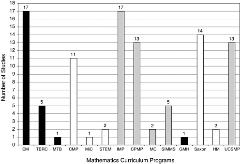
FIGURE 5-1 The distribution of comparative studies across programs. Programs are coded by grade band: black bars = elementary, white bars = middle grades, and gray bars = secondary. In this figure, there are six studies that involved two programs and one study that involved three programs.

NOTE: Five programs (MathScape, MMAP, MMOW/ARISE, Addison-Wesley, and Harcourt) are not shown above since no comparative studies were reviewed.

particular curricular program evaluations, in which case all 19 programs are listed separately. At other times, when we seek to inform ourselves on policy-related issues of funding and evaluating curricular materials, we use the NSF-supported, commercially generated, and UCSMP distinctions. We remind the reader of the artificial aspects of this distinction because at the present time, 18 of the 19 curricula are published commercially. In order to track the question of historical inception and policy implications, a distinction is drawn between the three categories. Figure 5-1 shows the distribution of comparative studies across the 14 programs.

The first result the committee wishes to report is the uneven distribution of studies across the curricula programs. There were 67 coded studies of the NSF curricula, 11 studies of UCSMP, and 17 studies of the commercial publishers. The 14 evaluation studies conducted on the Saxon materials compose the bulk of these 17-non-UCSMP and non-NSF-supported curricular evaluation studies. As these results suggest, we know more about the

evaluations of the NSF-supported curricula and UCSMP than about the evaluations of the commercial programs. We suggest that three factors account for this uneven distribution of studies. First, evaluations have been funded by the NSF both as a part of the original call, and as follow-up to the work in the case of three supplemental awards to two of the curricula programs. Second, most NSF-supported programs and UCSMP were developed at university sites where there is access to the resources of graduate students and research staff. Finally, there was some reported reluctance on the part of commercial companies to release studies that could affect perceptions of competitive advantage. As Figure 5-1 shows, there were quite a few comparative studies of Everyday Mathematics (EM), Connected Mathematics Project (CMP), Contemporary Mathematics in Context (Core-Plus Mathematics Project [CPMP]), Interactive Mathematics Program (IMP), UCSMP, and Saxon.

In the programs with many studies, we note that a significant number of studies were generated by a core set of authors. In some cases, the evaluation reports follow a relatively uniform structure applied to single schools, generating multiple studies or following cohorts over years. Others use a standardized evaluation approach to evaluate sequential courses. Any reports duplicating exactly the same sample, outcome measures, or forms of analysis were eliminated. For example, one study of Mathematics Trailblazers (Carter et al., 2002) reanalyzed the data from the larger ARC Implementation Center study (Sconiers et al., 2002), so it was not included separately. Synthesis studies referencing a variety of evaluation reports are summarized in Chapter 6 , but relevant individual studies that were referenced in them were sought out and included in this comparative review.

Other less formal comparative studies are conducted regularly at the school or district level, but such studies were not included in this review unless we could obtain formal reports of their results, and the studies met the criteria outlined for inclusion in our database. In our conclusions, we address the issue of how to collect such data more systematically at the district or state level in order to subject the data to the standards of scholarly peer review and make it more systematically and fairly a part of the national database on curricular effectiveness.

A standard for evaluation of any social program requires that an impact assessment is warranted only if two conditions are met: (1) the curricular program is clearly specified, and (2) the intervention is well implemented. Absent this assurance, one must have a means of ensuring or measuring treatment integrity in order to make causal inferences. Rossi et al. (1999, p. 238) warned that:

two prerequisites [must exist] for assessing the impact of an intervention. First, the program’s objectives must be sufficiently well articulated to make

it possible to specify credible measures of the expected outcomes, or the evaluator must be able to establish such a set of measurable outcomes. Second, the intervention should be sufficiently well implemented that there is no question that its critical elements have been delivered to appropriate targets. It would be a waste of time, effort, and resources to attempt to estimate the impact of a program that lacks measurable outcomes or that has not been properly implemented. An important implication of this last consideration is that interventions should be evaluated for impact only when they have been in place long enough to have ironed out implementation problems.

These same conditions apply to evaluation of mathematics curricula. The comparative studies in this report varied in the quality of documentation of these two conditions; however, all addressed them to some degree or another. Initially by reviewing the studies, we were able to identify one general design template, which consisted of seven critical decision points and determined that it could be used to develop a framework for conducting our meta-analysis. The seven critical decision points we identified initially were:

Choice of type of design: experimental or quasi-experimental;

For those studies that do not use random assignment: what methods of establishing comparability of groups were built into the design—this includes student characteristics, teacher characteristics, and the extent to which professional development was involved as part of the definition of a curriculum;

Definition of the appropriate unit of analysis (students, classes, teachers, schools, or districts);

Inclusion of an examination of implementation components;

Definition of the outcome measures and disaggregated results by program;

The choice of statistical tests, including statistical significance levels and effect size; and

Recognition of limitations to generalizability resulting from design choices.

These are critical decisions that affect the quality of an evaluation. We further identified a subset of these evaluation studies that met a set of minimum conditions that we termed at least minimally methodologically adequate studies. Such studies are those with the greatest likelihood of shedding light on the effectiveness of these programs. To be classified as at least minimally methodologically adequate, and therefore to be considered for further analysis, each evaluation study was required to:

Include quantifiably measurable outcomes such as test scores, responses to specified cognitive tasks of mathematical reasoning, performance evaluations, grades, and subsequent course taking; and

Provide adequate information to judge the comparability of samples. In addition, a study must have included at least one of the following additional design elements:

A report of implementation fidelity or professional development activity;

Results disaggregated by content strands or by performance by student subgroups; and/or

Multiple outcome measures or precise theoretical analysis of a measured construct, such as number sense, proof, or proportional reasoning.

Using this rubric, the committee identified a subset of 63 comparative studies to classify as at least minimally methodologically adequate and to analyze in depth to inform the conduct of future evaluations. There are those who would argue that any threat to the validity of a study discredits the findings, thus claiming that until we know everything, we know nothing. Others would claim that from the myriad of studies, examining patterns of effects and patterns of variation, one can learn a great deal, perhaps tentatively, about programs and their possible effects. More importantly, we can learn about methodologies and how to concentrate and focus to increase the likelihood of learning more quickly. As Lipsey (1997, p. 22) wrote:

In the long run, our most useful and informative contribution to program managers and policy makers and even to the evaluation profession itself may be the consolidation of our piecemeal knowledge into broader pictures of the program and policy spaces at issue, rather than individual studies of particular programs.

We do not wish to imply that we devalue studies of student affect or conceptions of mathematics, but decided that unless these indicators were connected to direct indicators of student learning, we would eliminate them from further study. As a result of this sorting, we eliminated 19 studies of NSF-supported curricula and 13 studies of commercially generated curricula. Of these, 4 were eliminated for their sole focus on affect or conceptions, 3 were eliminated for their comparative focus on outcomes other than achievement, such as teacher-related variables, and 19 were eliminated for their failure to meet the minimum additional characteristics specified in the criteria above. In addition, six others were excluded from the studies of commercial materials because they were not conducted within the grade-

level band specified by the committee for the selection of that program. From this point onward, all references can be assumed to refer to at least minimally methodologically adequate unless a study is referenced for illustration, in which case we label it with “EX” to indicate that it is excluded in the summary analyses. Studies labeled “EX” are occasionally referenced because they can provide useful information on certain aspects of curricular evaluation, but not on the overall effectiveness.

The at least minimally methodologically adequate studies reported on a variety of grade levels. Figure 5-2 shows the different grade levels of the studies. At times, the choice of grade levels was dictated by the years in which high-stakes tests were given. Most of the studies reported on multiple grade levels, as shown in Figure 5-2 .

Using the seven critical design elements of at least minimally methodologically adequate studies as a design template, we describe the overall database and discuss the array of choices on critical decision points with examples. Following that, we report on the results on the at least minimally methodologically adequate studies by program type. To do so, the results of each study were coded as either statistically significant or not. Those studies

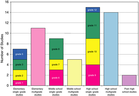
FIGURE 5-2 Single-grade studies by grade and multigrade studies by grade band.

that contained statistically significant results were assigned a percentage of outcomes that are positive (in favor of the treatment curriculum) based on the number of statistically significant comparisons reported relative to the total number of comparisons reported, and a percentage of outcomes that are negative (in favor of the comparative curriculum). The remaining were coded as the percentage of outcomes that are non significant. Then, using seven critical decision points as filters, we identified and examined more closely sets of studies that exhibited the strongest designs, and would therefore be most likely to increase our confidence in the validity of the evaluation. In this last section, we consider alternative hypotheses that could explain the results.

The committee emphasizes that we did not directly evaluate the materials. We present no analysis of results aggregated across studies by naming individual curricular programs because we did not consider the magnitude or rigor of the database for individual programs substantial enough to do so. Nevertheless, there are studies that provide compelling data concerning the effectiveness of the program in a particular context. Furthermore, we do report on individual studies and their results to highlight issues of approach and methodology and to remain within our primary charge, which was to evaluate the evaluations, we do not summarize results of the individual programs.

DESCRIPTION OF COMPARATIVE STUDIES DATABASE ON CRITICAL DECISION POINTS

An experimental or quasi-experimental design.

We separated the studies into experimental and quasiexperimental, and found that 100 percent of the studies were quasiexperimental (Campbell and Stanley, 1966; Cook and Campbell, 1979; and Rossi et al., 1999). 1 Within the quasi-experimental studies, we identified three subcategories of comparative study. In the first case, we identified a study as cross-curricular comparative if it compared the results of curriculum A with curriculum B. A few studies in this category also compared two samples within the curriculum to each other and specified different conditions such as high and low implementation quality.

A second category of a quasi-experimental study involved comparisons that could shed light on effectiveness involving time series studies. These studies compared the performance of a sample of students in a curriculum

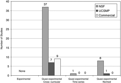
FIGURE 5-3 The number of comparative studies in each category.

under investigation across time, such as in a longitudinal study of the same students over time. A third category of comparative study involved a comparison to some form of externally normed results, such as populations taking state, national, or international tests or prior research assessment from a published study or studies. We categorized these studies and divided them into NSF, UCSMP, and commercial and labeled them by the categories above ( Figure 5-3 ).

In nearly all studies in the comparative group, the titles of experimental curricula were explicitly identified. The only exception to this was the ARC Implementation Center study (Sconiers et al., 2002), where three NSF-supported elementary curricula were examined, but in the results, their effects were pooled. In contrast, in the majority of the cases, the comparison curriculum is referred to simply as “traditional.” In only 22 cases were comparisons made between two identified curricula. Many others surveyed the array of curricula at comparison schools and reported on the most frequently used, but did not identify a single curriculum. This design strategy is used often because other factors were used in selecting comparison groups, and the additional requirement of a single identified curriculum in

these sites would often make it difficult to match. Studies were categorized into specified (including a single or multiple identified curricula) and nonspecified curricula. In the 63 studies, the central group was compared to an NSF-supported curriculum (1), an unnamed traditional curriculum (41), a named traditional curriculum (19), and one of the six commercial curricula (2). To our knowledge, any systematic impact of such a decision on results has not been studied, but we express concern that when a specified curriculum is compared to an unspecified content which is a set of many informal curriculum, the comparison may favor the coherency and consistency of the single curricula, and we consider this possibility subsequently under alternative hypotheses. We believe that a quality study should at least report the array of curricula that comprise the comparative group and include a measure of the frequency of use of each, but a well-defined alternative is more desirable.

If a study was both longitudinal and comparative, then it was coded as comparative. When studies only examined performances of a group over time, such as in some longitudinal studies, it was coded as quasi-experimental normed. In longitudinal studies, the problems created by student mobility were evident. In one study, Carroll (2001), a five-year longitudinal study of Everyday Mathematics, the sample size began with 500 students, 24 classrooms, and 11 schools. By 2nd grade, the longitudinal sample was 343. By 3rd grade, the number of classes increased to 29 while the number of original students decreased to 236 students. At the completion of the study, approximately 170 of the original students were still in the sample. This high rate of attrition from the study suggests that mobility is a major challenge in curricular evaluation, and that the effects of curricular change on mobile students needs to be studied as a potential threat to the validity of the comparison. It is also a challenge in curriculum implementation because students coming into a program do not experience its cumulative, developmental effect.

Longitudinal studies also have unique challenges associated with outcome measures, a study by Romberg et al. (in press) (EX) discussed one approach to this problem. In this study, an external assessment system and a problem-solving assessment system were used. In the External Assessment System, items from the National Assessment of Educational Progress (NAEP) and Third International Mathematics and Science Survey (TIMSS) were balanced across four strands (number, geometry, algebra, probability and statistics), and 20 items of moderate difficulty, called anchor items, were repeated on each grade-specific assessment (p. 8). Because the analyses of the results are currently under way, the evaluators could not provide us with final results of this study, so it is coded as EX.

However, such longitudinal studies can provide substantial evidence of the effects of a curricular program because they may be more sensitive to an

TABLE 5-1 Scores in Percentage Correct by Everyday Mathematics Students and Various Comparison Groups Over a Five-Year Longitudinal Study

accumulation of modest effects and/or can reveal whether the rates of learning change over time within curricular change.

The longitudinal study by Carroll (2001) showed that the effects of curricula may often accrue over time, but measurements of achievement present challenges to drawing such conclusions as the content and grade level change. A variety of measures were used over time to demonstrate growth in relation to comparison groups. The author chose a set of measures used previously in studies involving two Asian samples and an American sample to provide a contrast to the students in EM over time. For 3rd and 4th grades, where the data from the comparison group were not available, the authors selected items from the NAEP to bridge the gap. Table 5-1 summarizes the scores of the different comparative groups over five years. Scores are reported as the mean percentage correct for a series of tests on number computation, number concepts and applications, geometry, measurement, and data analysis.

It is difficult to compare performances on different tests over different groups over time against a single longitudinal group from EM, and it is not possible to determine whether the students’ performance is increasing or whether the changes in the tests at each grade level are producing the results; thus the results from longitudinal studies lacking a control group or use of sophisticated methodological analysis may be suspect and should be interpreted with caution.

In the Hirsch and Schoen (2002) study, based on a sample of 1,457 students, scores on Ability to Do Quantitative Thinking (ITED-Q) a subset of the Iowa Tests of Education Development, students in Core-Plus showed increasing performance over national norms over the three-year time period. The authors describe the content of the ITED-Q test and point out

that “although very little symbolic algebra is required, the ITED-Q is quite demanding for the full range of high school students” (p. 3). They further point out that “[t]his 3-year pattern is consistent, on average, in rural, urban, and suburban schools, for males and females, for various minority groups, and for students for whom English was not their first language” (p. 4). In this case, one sees that studies over time are important as results over shorter periods may mask cumulative effects of consistent and coherent treatments and such studies could also show increases that do not persist when subject to longer trajectories. One approach to longitudinal studies was used by Webb and Dowling in their studies of the Interactive Mathematics Program (Webb and Dowling, 1995a, 1995b, 1995c). These researchers conducted transcript analyses as a means to examine student persistence and success in subsequent course taking.

The third category of quasi-experimental comparative studies measured student outcomes on a particular curricular program and simply compared them to performance on national tests or international tests. When these tests were of good quality and were representative of a genuine sample of a relevant population, such as NAEP reports or TIMSS results, the reports often provided one a reasonable indicator of the effects of the program if combined with a careful description of the sample. Also, sometimes the national tests or state tests used were norm-referenced tests producing national percentiles or grade-level equivalents. The normed studies were considered of weaker quality in establishing effectiveness, but were still considered valid as examples of comparing samples to populations.

For Studies That Do Not Use Random Assignment: What Methods of Establishing Comparability Across Groups Were Built into the Design

The most fundamental question in an evaluation study is whether the treatment has had an effect on the chosen criterion variable. In our context, the treatment is the curriculum materials, and in some cases, related professional development, and the outcome of interest is academic learning. To establish if there is a treatment effect, one must logically rule out as many other explanations as possible for the differences in the outcome variable. There is a long tradition on how this is best done, and the principle from a design point of view is to assure that there are no differences between the treatment conditions (especially in these evaluations, often there are only the new curriculum materials to be evaluated and a control group) either at the outset of the study or during the conduct of the study.

To ensure the first condition, the ideal procedure is the random assignment of the appropriate units to the treatment conditions. The second condition requires that the treatment is administered reliably during the length of the study, and is assured through the careful observation and

control of the situation. Without randomization, there are a host of possible confounding variables that could differ among the treatment conditions and that are related themselves to the outcome variables. Put another way, the treatment effect is a parameter that the study is set up to estimate. Statistically, an estimate that is unbiased is desired. The goal is that its expected value over repeated samplings is equal to the true value of the parameter. Without randomization at the onset of a study, there is no way to assure this property of unbiasness. The variables that differ across treatment conditions and are related to the outcomes are confounding variables, which bias the estimation process.

Only one study we reviewed, Peters (1992), used randomization in the assignment of students to treatments, but that occurred because the study was limited to one teacher teaching two sections and included substantial qualitative methods, so we coded it as quasi-experimental. Others report partially assigning teachers randomly to treatment conditions (Thompson, et al., 2001; Thompson et al., 2003). Two primary reasons seem to account for a lack of use of pure experimental design. To justify the conduct and expense of a randomized field trial, the program must be described adequately and there must be relative assurance that its implementation has occurred over the duration of the experiment (Peterson et al., 1999). Additionally, one must be sure that the outcome measures are appropriate for the range of performances in the groups and valid relative to the curricula under investigation. Seldom can such conditions be assured for all students and teachers and over the duration of a year or more.

A second reason is that random assignment of classrooms to curricular treatment groups typically is not permitted or encouraged under normal school conditions. As one evaluator wrote, “Building or district administrators typically identified teachers who would be in the study and in only a few cases was random assignment of teachers to UCSMP Algebra or comparison classes possible. School scheduling and teacher preference were more important factors to administrators and at the risk of losing potential sites, we did not insist on randomization” (Mathison et al., 1989, p. 11).

The Joint Committee on Standards for Educational Evaluation (1994, p. 165) committee of evaluations recognized the likelihood of limitations on randomization, writing:

The groups being compared are seldom formed by random assignment. Rather, they tend to be natural groupings that are likely to differ in various ways. Analytical methods may be used to adjust for these initial differences, but these methods are based upon a number of assumptions. As it is often difficult to check such assumptions, it is advisable, when time and resources permit, to use several different methods of analysis to determine whether a replicable pattern of results is obtained.

Does the dearth of pure experimentation render the results of the studies reviewed worthless? Bias is not an “either-or” proposition, but it is a quantity of varying degrees. Through careful measurement of the most salient potential confounding variables, precise theoretical description of constructs, and use of these methods of statistical analysis, it is possible to reduce the amount of bias in the estimated treatment effect. Identification of the most likely confounding variables and their measurement and subsequent adjustments can greatly reduce bias and help estimate an effect that is likely to be more reflective of the true value. The theoretical fully specified model is an alternative to randomization by including relevant variables and thus allowing the unbiased estimation of the parameter. The only problem is realizing when the model is fully specified.

We recognized that we can never have enough knowledge to assure a fully specified model, especially in the complex and unstable conditions of schools. However, a key issue in determining the degree of confidence we have in these evaluations is to examine how they have identified, measured, or controlled for such confounding variables. In the next sections, we report on the methods of the evaluators in identifying and adjusting for such potential confounding variables.

One method to eliminate confounding variables is to examine the extent to which the samples investigated are equated either by sample selection or by methods of statistical adjustments. For individual students, there is a large literature suggesting the importance of social class to achievement. In addition, prior achievement of students must be considered. In the comparative studies, investigators first identified participation of districts, schools, or classes that could provide sufficient duration of use of curricular materials (typically two years or more), availability of target classes, or adequate levels of use of program materials. Establishing comparability was a secondary concern.

These two major factors were generally used in establishing the comparability of the sample:

Student population characteristics, such as demographic characteristics of students in terms of race/ethnicity, economic levels, or location type (urban, suburban, or rural).

Performance-level characteristics such as performance on prior tests, pretest performance, percentage passing standardized tests, or related measures (e.g., problem solving, reading).

In general, four methods of comparing groups were used in the studies we examined, and they permit different degrees of confidence in their results. In the first type, a matching class, school, or district was identified.

Studies were coded as this type if specified characteristics were used to select the schools systematically. In some of these studies, the methodology was relatively complex as correlates of performance on the outcome measures were found empirically and matches were created on that basis (Schneider, 2000; Riordan and Noyce, 2001; and Sconiers et al., 2002). For example, in the Sconiers et al. study, where the total sample of more than 100,000 students was drawn from five states and three elementary curricula are reviewed (Everyday Mathematics, Math Trailblazers [MT], and Investigations [IN], a highly systematic method was developed. After defining eligibility as a “reform school,” evaluators conducted separate regression analyses for the five states at each tested grade level to identify the strongest predictors of average school mathematics score. They reported, “reading score and low-income variables … consistently accounted for the greatest percentage of total variance. These variables were given the greatest weight in the matching process. Other variables—such as percent white, school mobility rate, and percent with limited English proficiency (LEP)—accounted for little of the total variance but were typically significant. These variables were given less weight in the matching process” (Sconiers et al., 2002, p. 10). To further provide a fair and complete comparison, adjustments were made based on regression analysis of the scores to minimize bias prior to calculating the difference in scores and reporting effect sizes. In their results the evaluators report, “The combined state-grade effect sizes for math and total are virtually identical and correspond to a percentile change of about 4 percent favoring the reform students” (p. 12).

A second type of matching procedure was used in the UCSMP evaluations. For example, in an evaluation centered on geometry learning, evaluators advertised in NCTM and UCSMP publications, and set conditions for participation from schools using their program in terms of length of use and grade level. After selecting schools with heterogeneous grouping and no tracking, the researchers used a match-pair design where they selected classes from the same school on the basis of mathematics ability. They used a pretest to determine this, and because the pretest consisted of two parts, they adjusted their significance level using the Bonferroni method. 2 Pairs were discarded if the differences in means and variance were significant for all students or for those students completing all measures, or if class sizes became too variable. In the algebra study, there were 20 pairs as a result of the matching, and because they were comparing three experimental conditions—first edition, second edition, and comparison classes—in the com-

parison study relevant to this review, their matching procedure identified 8 pairs. When possible, teachers were assigned randomly to treatment conditions. Most results are presented with the eight identified pairs and an accumulated set of means. The outcomes of this particular study are described below in a discussion of outcome measures (Thompson et al., 2003).

A third method was to measure factors such as prior performance or socio-economic status (SES) based on pretesting, and then to use analysis of covariance or multiple regression in the subsequent analysis to factor in the variance associated with these factors. These studies were coded as “control.” A number of studies of the Saxon curricula used this method. For example, Rentschler (1995) conducted a study of Saxon 76 compared to Silver Burdett with 7th graders in West Virginia. He reported that the groups differed significantly in that the control classes had 65 percent of the students on free and reduced-price lunch programs compared to 55 percent in the experimental conditions. He used scores on California Test of Basic Skills mathematics computation and mathematics concepts and applications as his pretest scores and found significant differences in favor of the experimental group. His posttest scores showed the Saxon experimental group outperformed the control group on both computation and concepts and applications. Using analysis of covariance, the computation difference in favor of the experimental group was statistically significant; however, the difference in concepts and applications was adjusted to show no significant difference at the p < .05 level.

A fourth method was noted in studies that used less rigorous methods of selection of sample and comparison of prior achievement or similar demographics. These studies were coded as “compare.” Typically, there was no explicit procedure to decide if the comparison was good enough. In some of the studies, it appeared that the comparison was not used as a means of selection, but rather as a more informal device to convince the reader of the plausibility of the equivalence of the groups. Clearly, the studies that used a more precise method of selection were more likely to produce results on which one’s confidence in the conclusions is greater.

Definition of Unit of Analysis

A major decision in forming an evaluation design is the unit of analysis. The unit of selection or randomization used to assign elements to treatment and control groups is closely linked to the unit of analysis. As noted in the National Research Council (NRC) report (1992, p. 21):

If one carries out the assignment of treatments at the level of schools, then that is the level that can be justified for causal analysis. To analyze the results at the student level is to introduce a new, nonrandomized level into

the study, and it raises the same issues as does the nonrandomized observational study…. The implications … are twofold. First, it is advisable to use randomization at the level at which units are most naturally manipulated. Second, when the unit of observation is at a “lower” level of aggregation than the unit of randomization, then for many purposes the data need to be aggregated in some appropriate fashion to provide a measure that can be analyzed at the level of assignment. Such aggregation may be as simple as a summary statistic or as complex as a context-specific model for association among lower-level observations.

In many studies, inadequate attention was paid to the fact that the unit of selection would later become the unit of analysis. The unit of analysis, for most curriculum evaluators, needs to be at least the classroom, if not the school or even the district. The units must be independently responding units because instruction is a group process. Students are not independent, the classroom—even if the teachers work together in a school on instruction—is not entirely independent, so the school is the unit. Care needed to be taken to ensure that an adequate numbers of units would be available to have sufficient statistical power to detect important differences.

A curriculum is experienced by students in a group, and this implies that individual student responses and what they learn are correlated. As a result, the appropriate unit of assignment and analysis must at least be defined at the classroom or teacher level. Other researchers (Bryk et al., 1993) suggest that the unit might be better selected at an even higher level of aggregation. The school itself provides a culture in which the curriculum is enacted as it is influenced by the policies and assignments of the principal, by the professional interactions and governance exhibited by the teachers as a group, and by the community in which the school resides. This would imply that the school might be the appropriate unit of analysis. Even further, to the extent that such decisions about curriculum are made at the district level and supported through resources and professional development at that level, the appropriate unit could arguably be the district. On a more practical level, we found that arguments can be made for a variety of decisions on the selection of units, and what is most essential is to make a clear argument for one’s choice, to use the same unit in the analysis as in the sample selection process, and to recognize the potential limits to generalization that result from one’s decisions.

We would argue in all cases that reports of how sites are selected must be explicit in the evaluation report. For example, one set of evaluation studies selected sites by advertisements in a journal distributed by the program and in NCTM journals (UCSMP) (Thompson et al., 2001; Thompson et al., 2003). The samples in their studies tended to be affluent suburban populations and predominantly white populations. Other conditions of inclusion, such as frequency of use also might have influenced this outcome,

but it is important that over a set of studies on effectiveness, all populations of students be adequately sampled. When a study is not randomized, adjustments for these confounding variables should be included. In our analysis of equity, we report on the concerns about representativeness of the overall samples and their impact on the generalizability of the results.

Implementation Components

The complexity of doing research on curricular materials introduces a number of possible confounding variables. Due to the documented complexity of curricular implementation, most comparative study evaluators attempt to monitor implementation in some fashion. A valuable outcome of a well-conducted evaluation is to determine not only if the experimental curriculum could ideally have a positive impact on learning, but whether it can survive or thrive in the conditions of schooling that are so variable across sites. It is essential to know what the treatment was, whether it occurred, and if so, to what degree of intensity, fidelity, duration, and quality. In our model in Chapter 3 , these factors were referred to as “implementation components.” Measuring implementation can be costly for large-scale comparative studies; however, many researchers have shown that variation in implementation is a key factor in determining effectiveness. In coding the comparative studies, we identified three types of components that help to document the character of the treatment: implementation fidelity, professional development treatments, and attention to teacher effects.

Implementation Fidelity

Implementation fidelity is a measure of the basic extent of use of the curricular materials. It does not address issues of instructional quality. In some studies, implementation fidelity is synonymous with “opportunity to learn.” In examining implementation fidelity, a variety of data were reported, including, most frequently, the extent of coverage of the curricular material, the consistency of the instructional approach to content in relation to the program’s theory, reports of pedagogical techniques, and the length of use of the curricula at the sample sites. Other less frequently used approaches documented the calendar of curricular coverage, requested teacher feedback by textbook chapter, conducted student surveys, and gauged homework policies, use of technology, and other particular program elements. Interviews with teachers and students, classroom surveys, and observations were the most frequently used data-gathering techniques. Classroom observations were conducted infrequently in these studies, except in cases when comparative studies were combined with case studies, typically with small numbers of schools and classes where observations

were conducted for long or frequent time periods. In our analysis, we coded only the presence or absence of one or more of these methods.

If the extent of implementation was used in interpreting the results, then we classified the study as having adjusted for implementation differences. Across all 63 at least minimally methodologically adequate studies, 44 percent reported some type of implementation fidelity measure, 3 percent reported and adjusted for it in interpreting their outcome measures, and 53 percent recorded no information on this issue. Differences among studies, by study type (NSF, UCSMP, and commercially generated), showed variation on this issue, with 46 percent of NSF reporting or adjusting for implementation, 75 percent of UCSMP, and only 11 percent of the other studies of commercial materials doing so. Of the commercial, non-UCSMP studies included, only one reported on implementation. Possibly, the evaluators for the NSF and UCSMP Secondary programs recognized more clearly that their programs demanded significant changes in practice that could affect their outcomes and could pose challenges to the teachers assigned to them.

A study by Abrams (1989) (EX) 3 on the use of Saxon algebra by ninth graders showed that concerns for implementation fidelity extend to all curricula, even those like Saxon whose methods may seem more likely to be consistent with common practice. Abrams wrote, “It was not the intent of this study to determine the effectiveness of the Saxon text when used as Saxon suggests, but rather to determine the effect of the text as it is being used in the classroom situations. However, one aspect of the research was to identify how the text is being taught, and how closely teachers adhere to its content and the recommended presentation” (p. 7). Her findings showed that for the 9 teachers and 300 students, treatment effects favoring the traditional group (using Dolciani’s Algebra I textbook, Houghton Mifflin, 1980) were found on the algebra test, the algebra knowledge/skills subtest, and the problem-solving test for this population of teachers (fixed effect). No differences were found between the groups on an algebra understanding/applications subtest, overall attitude toward mathematics, mathematical self-confidence, anxiety about mathematics, or enjoyment of mathematics. She suggests that the lack of differences might be due to the ways in which teachers supplement materials, change test conditions, emphasize

and deemphasize topics, use their own tests, vary the proportion of time spent on development and practice, use calculators and group work, and basically adapt the materials to their own interpretation and method. Many of these practices conflict directly with the recommendations of the authors of the materials.

A study by Briars and Resnick (2000) (EX) in Pittsburgh schools directly confronted issues relevant to professional development and implementation. Evaluators contrasted the performance of students of teachers with high and low implementation quality, and showed the results on two contrasting outcome measures, Iowa Test of Basic Skills (ITBS) and Balanced Assessment. Strong implementers were defined as those who used all of the EM components and provided student-centered instruction by giving students opportunities to explore mathematical ideas, solve problems, and explain their reasoning. Weak implementers were either not using EM or using it so little that the overall instruction in the classrooms was “hardly distinguishable from traditional mathematics instruction” (p. 8). Assignment was based on observations of student behavior in classes, the presence or absence of manipulatives, teacher questionnaires about the programs, and students’ knowledge of classroom routines associated with the program.

From the identification of strong- and weak-implementing teachers, strong- and weak-implementation schools were identified as those with strong- or weak-implementing teachers in 3rd and 4th grades over two consecutive years. The performance of students with 2 years of EM experience in these settings composed the comparative samples. Three pairs of strong- and weak-implementation schools with similar demographics in terms of free and reduced-price lunch (range 76 to 93 percent), student living with only one parent (range 57 to 82 percent), mobility (range 8 to 16 percent), and ethnicity (range 43 to 98 percent African American) were identified. These students’ 1st-grade ITBS scores indicated similarity in prior performance levels. Finally, evaluators predicted that if the effects were due to the curricular implementation and accompanying professional development, the effects on scores should be seen in 1998, after full implementation. Figure 5-4 shows that on the 1998 New Standards exams, placement in strong- and weak-implementation schools strongly affected students’ scores. Over three years, performance in the district on skills, concepts, and problem solving rose, confirming the evaluator’s predictions.

An article by McCaffrey et al. (2001) examining the interactions among instructional practices, curriculum, and student achievement illustrates the point that distinctions are often inadequately linked to measurement tools in their treatment of the terms traditional and reform teaching. In this study, researchers conducted an exploratory factor analysis that led them to create two scales for instructional practice: Reform Practices and Tradi-

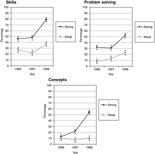
FIGURE 5-4 Percentage of students who met or exceeded the standard. Districtwide grade 4 New Standards Mathematics Reference Examination (NSMRE) performance for 1996, 1997, and 1998 by level of Everyday Mathematics implementation. Percentage of students who achieved the standard. Error bars denote the 99 percent confidence interval for each data point.

SOURCE: Re-created from Briars and Resnick (2000, pp. 19-20).

tional Practices. The reform scale measured the frequency, by means of teacher report, of teacher and student behaviors associated with reform instruction and assessment practices, such as using small-group work, explaining reasoning, representing and using data, writing reflections, or performing tasks in groups. The traditional scale focused on explanations to whole classes, the use of worksheets, practice, and short-answer assessments. There was a –0.32 correlation between scores for integrated curriculum teachers. There was a 0.27 correlation between scores for traditional

curriculum teachers. This shows that it is overly simplistic to think that reform and traditional practices are oppositional. The relationship among a variety of instructional practices is rather more complex as they interact with curriculum and various student populations.

Professional Development

Professional development and teacher effects were separated in our analysis from implementation fidelity. We recognized that professional development could be viewed by the readers of this report in two ways. As indicated in our model, professional development can be considered a program element or component or it can be viewed as part of the implementation process. When viewed as a program element, professional development resources are considered mandatory along with program materials. In relation to evaluation, proponents of considering professional development as a mandatory program element argue that curricular innovations, which involve the introduction of new topics, new types of assessment, or new ways of teaching, must make provision for adequate training, just as with the introduction of any new technology.

For others, the inclusion of professional development in the program elements without a concomitant inclusion of equal amounts of professional development relevant to a comparative treatment interjects a priori disproportionate treatments and biases the results. We hoped for an array of evaluation studies that might shed some empirical light on this dispute, and hence separated professional development from treatment fidelity, coding whether or not studies reported on the amount of professional development provided for the treatment and/or comparison groups. A study was coded as positive if it either reported on the professional development provided on the experimental group or reported the data on both treatments. Across all 63 at least minimally methodologically adequate studies, 27 percent reported some type of professional development measure, 1.5 percent reported and adjusted for it in interpreting their outcome measures, and 71.5 percent recorded no information on the issue.

A study by Collins (2002) (EX) 4 illustrates the critical and controversial role of professional development in evaluation. Collins studied the use of Connected Math over three years, in three middle schools in threat of being classified as low performing in the Massachusetts accountability system. A comparison was made between one school (School A) that engaged

substantively in professional development opportunities accompanying the program and two that did not (Schools B and C). In the CMP school reports (School A) totals between 100 and 136 hours of professional development were recorded for all seven teachers in grades 6 through 8. In School B, 66 hours were reported for two teachers and in School C, 150 hours were reported for eight teachers over three years. Results showed significant differences in the subsequent performance by students at the school with higher participation in professional development (School A) and it became a districtwide top performer; the other two schools remained at risk for low performance. No controls for teacher effects were possible, but the results do suggest the centrality of professional development for successful implementation or possibly suggest that the results were due to professional development rather than curriculum materials. The fact that these two interpretations cannot be separated is a problem when professional development is given to one and not the other. The effect could be due to textbook or professional development or an interaction between the two. Research designs should be adjusted to consider these issues when different conditions of professional development are provided.

Teacher Effects

These studies make it obvious that there are potential confounding factors of teacher effects. Many evaluation studies devoted inadequate attention to the variable of teacher quality. A few studies (Goodrow, 1998; Riordan and Noyce, 2001; Thompson et al., 2001; and Thompson et al., 2003) reported on teacher characteristics such as certification, length of service, experience with curricula, or degrees completed. Those studies that matched classrooms and reported by matched results rather than aggregated results sought ways to acknowledge the large variations among teacher performance and its impact on student outcomes. We coded any effort to report on possible teacher effects as one indicator of quality. Across all 63 at least minimally methodologically adequate studies, 16 percent reported some type of teacher effect measure, 3 percent reported and adjusted for it in interpreting their outcome measures, and 81 percent recorded no information on this issue.

One can see that the potential confounding factors of teacher effects, in terms of the provision of professional development or the measure of teacher effects, are not adequately considered in most evaluation designs. Some studies mention and give a subjective judgment as to the nature of the problem, but this is descriptive at the most. Hardly any of the studies actually do anything analytical, and because these are such important potential confounding variables, this presents a serious challenge to the efficacy of these studies. Figure 5-5 shows how attention to these factors varies

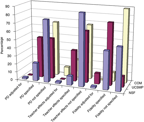
FIGURE 5-5 Treatment of implementation components by program type.

NOTE: PD = professional development.

across program categories among NSF-supported, UCSMP, and studies of commercial materials. In general, evaluations of NSF-supported studies were the most likely to measure these variables; UCSMP had the most standardized use of methods to do so across studies; and commercial material evaluators seldom reported on issues of implementation fidelity.

Identification of a Set of Outcome Measures and Forms of Disaggregation

Using the selected student outcomes identified in the program theory, one must conduct an impact assessment that refers to the design and measurement of student outcomes. In addition to selecting what outcomes should be measured within one’s program theory, one must determine how these outcomes are measured, when those measures are collected, and what

purpose they serve from the perspective of the participants. In the case of curricular evaluation, there are significant issues involved in how these measures are reported. To provide insight into the level of curricular validity, many evaluators prefer to report results by topic, content strand, or item cluster. These reports often present the level of specificity of outcome needed to inform curriculum designers, especially when efforts are made to document patterns of errors, distribution of results across multiple choices, or analyses of student methods. In these cases, whole test scores may mask essential differences in impact among curricula at the level of content topics, reporting only average performance.

On the other hand, many large-scale assessments depend on methods of test equating that rely on whole test scores and make comparative interpretations of different test administrations by content strands of questionable reliability. Furthermore, there are questions such as whether to present only gain scores effect sizes, how to link pretests and posttests, and how to determine the relative curricular sensitivity of various outcome measures.

The findings of comparative studies are reported in terms of the outcome measure(s) collected. To describe the nature of the database with regard to outcome measures and to facilitate our analyses of the studies, we classified each of the included studies on four outcome measure dimensions:

Total score reported;

Disaggregation of content strands, subtest, performance level, SES, or gender;

Outcome measure that was specific to curriculum; and

Use of multiple outcome measures.

Most studies reported a total score, but we did find studies that reported only subtest scores or only scores on an item-by-item basis. For example, in the Ben-Chaim et al. (1998) evaluation study of Connected Math, the authors were interested in students’ proportional reasoning proficiency as a result of use of this curriculum. They asked students from eight seventh-grade classes of CMP and six seventh-grade classes from the control group to solve a variety of tasks categorized as rate and density problems. The authors provide precise descriptions of the cognitive challenges in the items; however, they do not explain if the problems written up were representative of performance on a larger set of items. A special rating form was developed to code responses in three major categories (correct answer, incorrect answer, and no response), with subcategories indicating the quality of the work that accompanied the response. No reports on reliability of coding were given. Performance on standardized tests indicated that control students’ scores were slightly higher than CMP at the beginning of the

year and lower at the end. Twenty-five percent of the experimental group members were interviewed about their approaches to the problems. The CMP students outperformed the control students (53 percent versus 28 percent) overall in providing the correct answers and support work, and 27 percent of the control group gave an incorrect answer or showed incorrect thinking compared to 13 percent of the CMP group. An item-level analysis permitted the researchers to evaluate the actual strategies used by the students. They reported, for example, that 82 percent of CMP students used a “strategy focused on package price, unit price, or a combination of the two; those effective strategies were used by only 56 of 91 control students (62 percent)” (p. 264).

The use of item or content strand-level comparative reports had the advantage that they permitted the evaluators to assess student learning strategies specific to a curriculum’s program theory. For example, at times, evaluators wanted to gauge the effectiveness of using problems different from those on typical standardized tests. In this case, problems were drawn from familiar circumstances but carefully designed to create significant cognitive challenges, and assess how well the informal strategies approach in CMP works in comparison to traditional instruction. The disadvantages of such an approach include the use of only a small number of items and the concerns for reliability in scoring. These studies seem to represent a method of creating hybrid research models that build on the detailed analyses possible using case studies, but still reporting on samples that provide comparative data. It possibly reflects the concerns of some mathematicians and mathematics educators that the effectiveness of materials needs to be evaluated relative to very specific, research-based issues on learning and that these are often inadequately measured by multiple-choice tests. However, a decision not to report total scores led to a trade-off in the reliability and representativeness of the reported data, which must be addressed to increase the objectivity of the reports.

Second, we coded whether outcome data were disaggregated in some way. Disaggregation involved reporting data on dimensions such as content strand, subtest, test item, ethnic group, performance level, SES, and gender. We found disaggregated results particularly helpful in understanding the findings of studies that found main effects, and also in examining patterns across studies. We report the results of the studies’ disaggregation by content strand in our reports of effects. We report the results of the studies’ disaggregation by subgroup in our discussions of generalizability.

Third, we coded whether a study used an outcome measure that the evaluator reported as being sensitive to a particular treatment—this is a subcategory of what was defined in our framework as “curricular validity of measures.” In such studies, the rationale was that readily available measures such as state-mandated tests, norm-referenced standardized tests, and

college entrance examinations do not measure some of the aims of the program under study. A frequently cited instance of this was that “off the shelf” instruments do not measure well students’ ability to apply their mathematical knowledge to problems embedded in complex settings. Thus, some studies constructed a collection of tasks that assessed this ability and collected data on it (Ben-Chaim et al., 1998; Huntley et al., 2000).

Finally, we recorded whether a study used multiple outcome measures. Some studies used a variety of achievement measures and other studies reported on achievement accompanied by measures such as subsequent course taking or various types of affective measures. For example, Carroll (2001, p. 47) reported results on a norm-referenced standardized achievement test as well as a collection of tasks developed in other studies.

A study by Huntley et al. (2000) illustrates how a variety of these techniques were combined in their outcome measures. They developed three assessments. The first emphasized contextualized problem solving based on items from the American Mathematical Association of Two-Year Colleges and others; the second assessment was on context-free symbolic manipulation and a third part requiring collaborative problem solving. To link these measures to the overall evaluation, they articulated an explicit model of cognition based on how one links an applied situation to mathematical activity through processes of formulation and interpretation. Their assessment strategy permitted them to investigate algebraic reasoning as an ability to use algebraic ideas and techniques to (1) mathematize quantitative problem situations, (2) use algebraic principles and procedures to solve equations, and (3) interpret results of reasoning and calculations.

In presenting their data comparing performance on Core-Plus and traditional curriculum, they presented both main effects and comparisons on subscales. Their design of outcome measures permitted them to examine differences in performance with and without context and to conclude with statements such as “This result illustrates that CPMP students perform better than control students when setting up models and solving algebraic problems presented in meaningful contexts while having access to calculators, but CPMP students do not perform as well on formal symbol-manipulation tasks without access to context cues or calculators” (p. 349). The authors go on to present data on the relationship between knowing how to plan or interpret solutions and knowing how to carry them out. The correlations between these variables were weak but significantly different (0.26 for control groups and 0.35 for Core-Plus). The advantage of using multiple measures carefully tied to program theory is that they can permit one to test fine content distinctions that are likely to be the level of adjustments necessary to fine tune and improve curricular programs.

Another interesting approach to the use of outcome measures is found in the UCSMP studies. In many of these studies, evaluators collected infor-

TABLE 5-2 Mean Percentage Correct on the Subject Tests

mation from teachers’ reports and chapter reviews as to whether topics for items on the posttests were taught, calling this an “opportunity to learn” measure. The authors reported results from three types of analyses: (1) total test scores, (2) fair test scores (scores reported by program but only on items on topics taught), and (3) conservative test scores (scores on common items taught in both). Table 5-2 reports on the variations across the multiple- choice test scores for the Geometry study (Thompson et al., 2003) on a standardized test, High School Subject Tests-Geometry Form B , and the UCSMP-constructed Geometry test, and for the Advanced Algebra Study on the UCSMP-constructed Advanced Algebra test (Thompson et al., 2001). The table shows the mean scores for UCSMP classes and comparison classes. In each cell, mean percentage correct is reported first by whole test, then by fair test, and then by conservative test.

The authors explicitly compare the items from the standard Geometry test with the items from the UCSMP test and indicate overlap and difference. They constructed their own test because, in their view, the standard test was not adequately balanced among skills, properties, and real-world uses. The UCSMP test included items on transformations, representations, and applications that were lacking in the national test. Only five items were taught by all teachers; hence in the case of the UCSMP geometry test, there is no report on a conservative test. In the Advanced Algebra evaluation, only a UCSMP-constructed test was viewed as appropriate to cover the treatment of the prior material and alignment to the goals of the new course. These data sets demonstrate the challenge of selecting appropriate outcome measures, the sensitivity of the results to those decisions, and the importance of full disclosure of decision-making processes in order to permit readers to assess the implications of the choices. The methodology utilized sought to ensure that the material in the course was covered adequately by treatment teachers while finding ways to make comparisons that reflected content coverage.

Only one study reported on its outcomes using embedded assessment items employed over the course of the year. In a study of Saxon and UCSMP, Peters (1992) (EX) studied the use of these materials with two classrooms taught by the same teacher. In this small study, he randomly assigned students to treatment groups and then measured their performance on four unit tests composed of items common to both curricula and their progress on the Orleans-Hanna Algebraic Prognosis Test.

Peters’ study showed no significant difference in placement scores between Saxon and UCSMP on the posttest, but did show differences on the embedded assessment. Figure 5-6 (Peters, 1992, p. 75) shows an interesting display of the differences on a “continuum” that shows both the direction and magnitude of the differences and provides a level of concept specificity missing in many reports. This figure and a display ( Figure 5-7 ) in a study by Senk (1991, p. 18) of students’ mean scores on Curriculum A versus Curriculum B with a 10 percent range of differences marked represent two excellent means to communicate the kinds of detailed content outcome information that promises to be informative to curriculum writers, publishers, and school decision makers. In Figure 5-7 , 16 items listed by number were taken from the Second International Mathematics Study. The Functions, Statistics, and Trigonometry sample averaged 41 percent correct on these items whereas the U.S. precalculus sample averaged 38 percent. As shown in the figure, differences of 10 percent or less fall inside the banded area and greater than 10 percent fall outside, producing a display that makes it easy for readers and designers to identify the relative curricular strengths and weaknesses of topics.

While we value detailed outcome measure information, we also recognize the importance of examining curricular impact on students’ standardized test performance. Many developers, but not all, are explicit in rejecting standardized tests as adequate measures of the outcomes of their programs, claiming that these tests focus on skills and manipulations, that they are overly reliant on multiple-choice questions, and that they are often poorly aligned to new content emphases such as probability and statistics, transformations, use of contextual problems and functions, and process skills, such as problem solving, representation, or use of calculators. However, national and state tests are being revised to include more content on these topics and to draw on more advanced reasoning. Furthermore, these high-stakes tests are of major importance in school systems, determining graduation, passing standards, school ratings, and so forth. For this reason, if a curricular program demonstrated positive impact on such measures, we referred to that in Chapter 3 as establishing “curricular alignment with systemic factors.” Adequate performance on these measures is of paramount importance to the survival of reform (to large groups of parents and

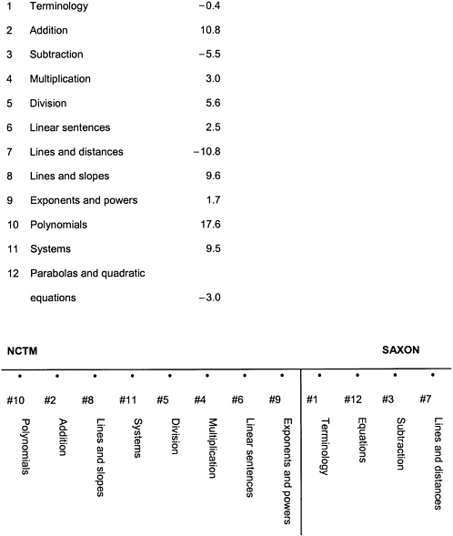
FIGURE 5-6 Continuum of criterion score averages for studied programs.

SOURCE: Peters (1992, p. 75).

school administrators). These examples demonstrate how careful attention to outcomes measures is an essential element of valid evaluation.

In Table 5-3 , we document the number of studies using a variety of types of outcome measures that we used to code the data, and also report on the types of tests used across the studies.

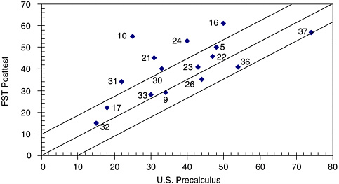
FIGURE 5-7 Achievement (percentage correct) on Second International Mathematics Study (SIMS) items by U.S. precalculus students and functions, statistics, and trigonometry (FST) students.

SOURCE: Re-created from Senk (1991, p. 18).

TABLE 5-3 Number of Studies Using a Variety of Outcome Measures by Program Type

A Choice of Statistical Tests, Including Statistical Significance and Effect Size

In our first review of the studies, we coded what methods of statistical evaluation were used by different evaluators. Most common were t-tests; less frequently one found Analysis of Variance (ANOVA), Analysis of Co-

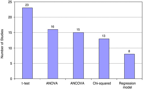
FIGURE 5-8 Statistical tests most frequently used.

variance (ANCOVA), and chi-square tests. In a few cases, results were reported using multiple regression or hierarchical linear modeling. Some used multiple tests; hence the total exceeds 63 ( Figure 5-8 ).

One of the difficult aspects of doing curriculum evaluations concerns using the appropriate unit both in terms of the unit to be randomly assigned in an experimental study and the unit to be used in statistical analysis in either an experimental or quasi-experimental study.

For our purposes, we made the decision that unless the study concerned an intact student population such as the freshman at a single university, where a student comparison was the correct unit, we believed that for statistical tests, the unit should be at least at the classroom level. Judgments were made for each study as to whether the appropriate unit was utilized. This question is an important one because statistical significance is related to sample size, and as a result, studies that inappropriately use the student as the unit of analysis could be concluding significant differences where they are not present. For example, if achievement differences between two curricula are tested in 16 classrooms with 400 students, it will always be easier to show significant differences using scores from those 400 students than using 16 classroom means.

Fifty-seven studies used students as the unit of analysis in at least one test of significance. Three of these were coded as correct because they involved whole populations. In all, 10 studies were coded as using the

TABLE 5-4 Performance on Applied Algebra Problems with Use of Calculators, Part 1

TABLE 5-5 Reanalysis of Algebra Performance Data

correct unit of analysis; hence, 7 studies used teachers or classes, or schools. For some studies where multiple tests were conducted, a judgment was made as to whether the primary conclusions drawn treated the unit of analysis adequately. For example, Huntley et al. (2000) compared the performance of CPMP students with students in a traditional course on a measure of ability to formulate and use algebraic models to answer various questions about relationships among variables. The analysis used students as the unit of analysis and showed a significant difference, as shown in Table 5-4 .

To examine the robustness of this result, we reanalyzed the data using an independent sample t-test and a matched pairs t-test with class means as the unit of analysis in both tests ( Table 5-5 ). As can be seen from the analyses, in neither statistical test was the difference between groups found to be significantly different (p < .05), thus emphasizing the importance of using the correct unit in analyzing the data.

Reanalysis of student-level data using class means will not always result

TABLE 5-6 Mean Percentage Correct on Entire Multiple-Choice Posttest: Second Edition and Non-UCSMP

in a change in finding. Furthermore, using class means as the unit of analysis does not suggest that significant differences will not be found. For example, a study by Thompson et al. (2001) compared the performance of UCSMP students with the performance of students in a more traditional program across several measures of achievement. They found significant differences between UCSMP students and the non-UCSMP students on several measures. Table 5-6 shows results of an analysis of a multiple-choice algebraic posttest using class means as the unit of analysis. Significant differences were found in five of eight separate classroom comparisons, as shown in the table. They also found a significant difference using a matched-pairs t-test on class means.

The lesson to be learned from these reanalyses is that the choice of unit of analysis and the way the data are aggregated can impact study findings in important ways including the extent to which these findings can be generalized. Thus it is imperative that evaluators pay close attention to such considerations as the unit of analysis and the way data are aggregated in the design, implementation, and analysis of their studies.

Second, effect size has become a relatively common and standard way of gauging the practical significance of the findings. Statistical significance only indicates whether the main-level differences between two curricula are large enough to not be due to chance, assuming they come from the same population. When statistical differences are found, the question remains as to whether such differences are large enough to consider. Because any innovation has its costs, the question becomes one of cost-effectiveness: Are the differences in student achievement large enough to warrant the costs of change? Quantifying the practical effect once statistical significance is established is one way to address this issue. There is a statistical literature for doing this, and for the purposes of this review, the committee simply noted whether these studies have estimated such an effect. However, the committee further noted that in conducting meta-analyses across these studies, effect size was likely to be of little value. These studies used an enormous variety of outcome measures, and even using effect size as a means to standardize units across studies is not sensible when the measures in each

study address such a variety of topics, forms of reasoning, content levels, and assessment strategies.

We note very few studies drew upon the advances in methodologies employed in modeling, which include causal modeling, hierarchical linear modeling (Bryk and Raudenbush, 1992; Bryk et al., 1993), and selection bias modeling (Heckman and Hotz, 1989). Although developing detailed specifications for these approaches is beyond the scope of this review, we wish to emphasize that these methodological advances should be considered within future evaluation designs.

Results and Limitations to Generalizability Resulting from Design Constraints

One also must consider what generalizations can be drawn from the results (Campbell and Stanley, 1966; Caporaso and Roos, 1973; and Boruch, 1997). Generalization is a matter of external validity in that it determines to what populations the study results are likely to apply. In designing an evaluation study, one must carefully consider, in the selection of units of analysis, how various characteristics of those units will affect the generalizability of the study. It is common for evaluators to conflate issues of representativeness for the purpose of generalizability (external validity) and comparativeness (the selection of or adjustment for comparative groups [internal validity]). Not all studies must be representative of the population served by mathematics curricula to be internally valid. But, to be generalizable beyond restricted communities, representativeness must be obtained by the random selection of the basic units. Clearly specifying such limitations to generalizability is critical. Furthermore, on the basis of equity considerations, one must be sure that if overall effectiveness is claimed, that the studies have been conducted and analyzed with reference of all relevant subgroups.

Thus, depending on the design of a study, its results may be limited in generalizability to other populations and circumstances. We identified four typical kinds of limitations on the generalizability of studies and coded them to determine, on the whole, how generalizable the results across studies might be.

First, there were studies whose designs were limited by the ability or performance level of the students in the samples. It was not unusual to find that when new curricula were implemented at the secondary level, schools kept in place systems of tracking that assigned the top students to traditional college-bound curriculum sequences. As a result, studies either used comparative groups who were matched demographically but less skilled than the population as a whole, in relation to prior learning, or their results compared samples of less well-prepared students to samples of students

with stronger preparations. Alternatively, some studies reported on the effects of curricula reform on gifted and talented students or on college-attending students. In these cases, the study results would also limit the generalizability of the results to similar populations. Reports using limited samples of students’ ability and prior performance levels were coded as a limitation to the generalizability of the study.

For example, Wasman (2000) conducted a study of one school (six teachers) and examined the students’ development of algebraic reasoning after one (n=100) and two years (n=73) in CMP. In this school, the top 25 percent of the students are counseled to take a more traditional algebra course, so her experimental sample, which was 61 percent white, 35 percent African American, 3 percent Asian, and 1 percent Hispanic, consisted of the lower 75 percent of the students. She reported on the student performance on the Iowa Algebraic Aptitude Test (IAAT) (1992), in the subcategories of interpreting information, translating symbols, finding relationships, and using symbols. Results for Forms 1 and 2 of the test, for the experimental and norm group, are shown in Table 5-7 for 8th graders.

In our coding of outcomes, this study was coded as showing no significant differences, although arguably its results demonstrate a positive set of

TABLE 5-7 Comparing Iowa Algebraic Aptitude Test (IAAT) Mean Scores of the Connected Mathematics Project Forms 1 and 2 to the Normative Group (8th Graders)

outcomes as the treatment group was weaker than the control group. Had the researcher used a prior achievement measure and a different statistical technique, significance might have been demonstrated, although potential teacher effects confound interpretations of results.

A second limitation to generalizability was when comparative studies resided entirely at curriculum pilot site locations, where such sites were developed as a means to conduct formative evaluations of the materials with close contact and advice from teachers. Typically, pilot sites have unusual levels of teacher support, whether it is in the form of daily technical support in the use of materials or technology or increased quantities of professional development. These sites are often selected for study because they have established cooperative agreements with the program developers and other sources of data, such as classroom observations, are already available. We coded whether the study was conducted at a pilot site to signal potential limitations in generalizability of the findings.

Third, studies were also coded as being of limited generalizability if they failed to disaggregate their data by socioeconomic class, race, gender, or some other potentially significant sources of restriction on the claims. We recorded the categories in which disaggregation occurred and compiled their frequency across the studies. Because of the need to open the pipeline to advanced study in mathematics by members of underrepresented groups, we were particularly concerned about gauging the extent to which evaluators factored such variables into their analysis of results and not just in terms of the selection of the sample.

Of the 46 included studies of NSF-supported curricula, 19 disaggregated their data by student subgroup. Nine of 17 studies of commercial materials disaggregated their data. Figure 5-9 shows the number of studies that disaggregated outcomes by race or ethnicity, SES, gender, LEP, special education status, or prior achievement. Studies using multiple categories of disaggregation were counted multiple times by program category.

The last category of restricted generalization occurred in studies of limited sample size. Although such studies may have provided more indepth observations of implementation and reports on professional development factors, the smaller numbers of classrooms and students in the study would limit the extent of generalization that could be drawn from it. Figure 5-10 shows the distribution of sizes of the samples in terms of numbers of students by study type.

Summary of Results by Student Achievement Among Program Types

We present the results of the studies as a means to further investigate their methodological implications. To this end, for each study, we counted across outcome measures the number of findings that were positive, nega-

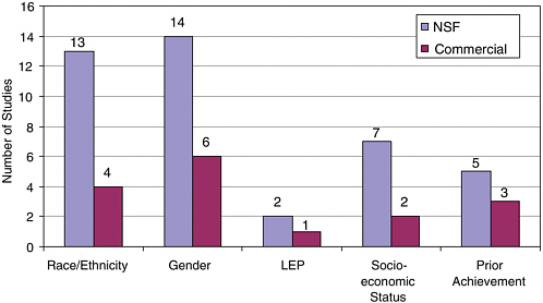
FIGURE 5-9 Disaggregation of subpopulations.

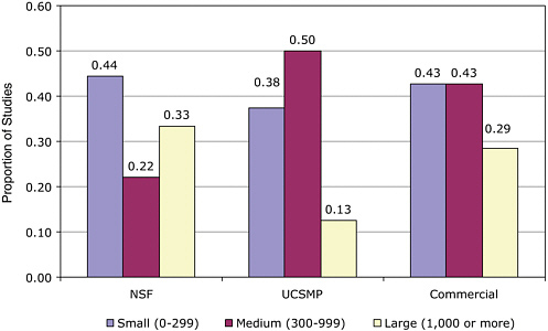
FIGURE 5-10 Proportion of studies by sample size and program.

tive, or indeterminate (no significant difference) and then calculated the proportion of each. We represented the calculation of each study as a triplet (a, b, c) where a indicates the proportion of the results that were positive and statistically significantly stronger than the comparison program, b indicates the proportion that were negative and statistically significantly weaker than the comparison program, and c indicates the proportion that showed no significant difference between the treatment and the comparative group. For studies with a single outcome measure, without disaggregation by content strand, the triplet is always composed of two zeros and a single one. For studies with multiple measures or disaggregation by content strand, the triplet is typically a set of three decimal values that sum to one. For example, a study with one outcome measure in favor of the experimental treatment would be coded (1, 0, 0), while one with multiple measures and mixed results more strongly in favor of the comparative curriculum might be listed as (.20, .50, .30). This triplet would mean that for 20 percent of the comparisons examined, the evaluators reported statistically significant positive results, for 50 percent of the comparisons the results were statistically significant in favor of the comparison group, and for 30 percent of the comparisons no significant difference were found. Overall, the mean score on these distributions was (.54, .07, .40), indicating that across all the studies, 54 percent of the comparisons favored the treatment, 7 percent favored the comparison group, and 40 percent showed no significant difference. Table 5-8 shows the comparison by curricular program types. We present the results by individual program types, because each program type relies on a similar program theory and hence could lead to patterns of results that would be lost in combining the data. If the studies of commercial materials are all grouped together to include UCSMP, their pattern of results is (.38, .11, .51). Again we emphasize that due to our call for increased methodological rigor and the use of multiple methods, this result is not sufficient to establish the curricular effectiveness of these programs as a whole with adequate certainty.

We caution readers that these results are summaries of the results presented across a set of evaluations that meet only the standard of at least

TABLE 5-8 Comparison by Curricular Program Types

minimally methodologically adequate . Calculations of statistical significance of each program’s results were reported by the evaluators; we have made no adjustments for weaknesses in the evaluations such as inappropriate use of units of analysis in calculating statistical significance. Evaluations that consistently used the correct unit of analysis, such as UCSMP, could have fewer reports of significant results as a consequence. Furthermore, these results are not weighted by study size. Within any study, the results pay no attention to comparative effect size or to the established credibility of an outcome measure. Similarly, these results do not take into account differences in the populations sampled, an important consideration in generalizing the results. For example, using the same set of studies as an example, UCSMP studies used volunteer samples who responded to advertisements in their newsletters, resulting in samples with disproportionately Caucasian subjects from wealthier schools compared to national samples. As a result, we would suggest that these results are useful only as baseline data for future evaluation efforts. Our purpose in calculating these results is to permit us to create filters from the critical decision points and test how the results change as one applies more rigorous standards.

Given that none of the studies adequately addressed all of the critical criteria, we do not offer these results as definitive, only suggestive—a hypothesis for further study. In effect, given the limitations of time and support, and the urgency of providing advice related to policy, we offer this filtering approach as an informal meta-analytic technique sufficient to permit us to address our primary task, namely, evaluating the quality of the evaluation studies.

This approach reflects the committee’s view that to deeply understand and improve methodology, it is necessary to scrutinize the results and to determine what inferences they provide about the conduct of future evaluations. Analogous to debates on consequential validity in testing, we argue that to strengthen methodology, one must consider what current methodologies are able (or not able) to produce across an entire series of studies. The remainder of the chapter is focused on considering in detail what claims are made by these studies, and how robust those claims are when subjected to challenge by alternative hypothesis, filtering by tests of increasing rigor, and examining results and patterns across the studies.

Alternative Hypotheses on Effectiveness

In the spirit of scientific rigor, the committee sought to consider rival hypotheses that could explain the data. Given the weaknesses in the designs generally, often these alternative hypotheses cannot be dismissed. However, we believed that only after examining the configuration of results and

alternative hypotheses can the next generation of evaluations be better informed and better designed. We began by generating alternative hypotheses to explain the positive directionality of the results in favor of experimental groups. Alternative hypotheses included the following:

The teachers in the experimental groups tended to be self-selecting early adopters, and thus able to achieve effects not likely in regular populations.

Changes in student outcomes reflect the effects of professional development instruction, or level of classroom support (in pilot sites), and thus inflate the predictions of effectiveness of curricular programs.

Hawthorne effect (Franke and Kaul, 1978) occurs when treatments are compared to everyday practices, due to motivational factors that influence experimental participants.

The consistent difference is due to the coherence and consistency of a single curricular program when compared to multiple programs.

The significance level is only achieved by the use of the wrong unit of analysis to test for significance.

Supplemental materials or new teaching techniques produce the results and not the experimental curricula.

Significant results reflect inadequate outcome measures that focus on a restricted set of activities.

The results are due to evaluator bias because too few evaluators are independent of the program developers.

At the same time, one could argue that the results actually underestimate the performance of these materials and are conservative measures, and their alternative hypotheses also deserve consideration:

Many standardized tests are not sensitive to these curricular approaches, and by eliminating studies focusing on affect, we eliminated a key indicator of the appeal of these curricula to students.

Poor implementation or increased demands on teachers’ knowledge dampens the effects.

Often in the experimental treatment, top-performing students are missing as they are advised to take traditional sequences, rendering the samples unequal.

Materials are not well aligned with universities and colleges because tests for placement and success in early courses focus extensively on algebraic manipulation.

Program implementation has been undercut by negative publicity and the fears of parents concerning change.

There are also a number of possible hypotheses that may be affecting the results in either direction, and we list a few of these:

Examining the role of the teacher in curricular decision making is an important element in effective implementation, and design mandates of evaluation design make this impossible (and the positives and negatives or single- versus dual-track curriculum as in Lundin, 2001).

Local tests that are sensitive to the curricular effects typically are not mandatory and hence may lead to unpredictable performance by students.

Different types and extent of professional development may affect outcomes differentially.

Persistence or attrition may affect the mean scores and are often not considered in the comparative analyses.

One could also generate reasons why the curricular programs produced results showing no significance when one program or the other is actually more effective. This could include high degrees of variability in the results, samples that used the correct unit of analysis but did not obtain consistent participation across enough cases, implementation that did not show enough fidelity to the measures, or outcome measures insensitive to the results. Again, subsequent designs should be better informed by these findings to improve the likelihood that they will produce less ambiguous results and replication of studies could also give more confidence in the findings.

It is beyond the scope of this report to consider each of these alternative hypotheses separately and to seek confirmation or refutation of them. However, in the next section, we describe a set of analyses carried out by the committee that permits us to examine and consider the impact of various critical evaluation design decisions on the patterns of outcomes across sets of studies. A number of analyses shed some light on various alternative hypotheses and may inform the conduct of future evaluations.

Filtering Studies by Critical Decision Points to Increase Rigor

In examining the comparative studies, we identified seven critical decision points that we believed would directly affect the rigor and efficacy of the study design. These decision points were used to create a set of 16 filters. These are listed as the following questions:

Was there a report on comparability relative to SES?

Was there a report on comparability of samples relative to prior knowledge?

Was there a report on treatment fidelity?

Was professional development reported on?

Was the comparative curriculum specified?

Was there any attempt to report on teacher effects?

Was a total test score reported?

Was total test score(s) disaggregated by content strand?

Did the outcome measures match the curriculum?

Were multiple tests used?

Was the appropriate unit of analysis used in their statistical tests?

Did they estimate effect size for the study?

Was the generalizability of their findings limited by use of a restricted range of ability levels?

Was the generalizability of their findings limited by use of pilot sites for their study?

Was the generalizability of their findings limited by not disaggregating their results by subgroup?

Was the generalizability of their findings limited by use of small sample size?

The studies were coded to indicate if they reported having addressed these considerations. In some cases, the decision points were coded dichotomously as present or absent in the studies, and in other cases, the decision points were coded trichotomously, as description presented, absent, or statistically adjusted for in the results. For example, a study may or may not report on the comparability of the samples in terms of race, ethnicity, or socioeconomic status. If a report on SES was given, the study was coded as “present” on this decision; if a report was missing, it was coded as “absent”; and if SES status or ethnicity was used in the analysis to actually adjust outcomes, it was coded as “adjusted for.” For each coding, the table that follows reports the number of studies that met that condition, and then reports on the mean percentage of statistically significant results, and results showing no significant difference for that set of studies. A significance test is run to see if the application of the filter produces changes in the probability that are significantly different. 5

In the cases in which studies are coded into three distinct categories—present, absent, and adjusted for—a second set of filters is applied. First, the studies coded as present or adjusted for are combined and compared to those coded as absent; this is what we refer to as a weak test of the rigor of the study. Second, the studies coded as present or absent are combined and compared to those coded as adjusted for. This is what we refer to as a strong test. For dichotomous codings, there can be as few as three compari-

sons, and for trichotomous codings, there can be nine comparisons with accompanying tests of significance. Trichotomous codes were used for adjustments for SES and prior knowledge, examining treatment fidelity, professional development, teacher effects, and reports on effect sizes. All others were dichotomous.

NSF Studies and the Filters

For example, there were 11 studies of NSF-supported curricula that simply reported on the issues of SES in creating equivalent samples for comparison, and for this subset the mean probabilities of getting positive, negative, or results showing no significant difference were (.47, .10, .43). If no report of SES was supplied (n= 21), those probabilities become (.57, .07, .37), indicating an increase in positive results and a decrease in results showing no significant difference. When an adjustment is made in outcomes based on differences in SES (n=14), the probabilities change to (.72, .00, .28), showing a higher likelihood of positive outcomes. The probabilities that result from filtering should always be compared back to the overall results of (.59, .06, .35) (see Table 5-8 ) so as to permit one to judge the effects of more rigorous methodological constraints. This suggests that a simple report on SES without adjustment is least likely to produce positive outcomes; that is, no report produces the outcomes next most likely to be positive and studies that adjusted for SES tend to have a higher proportion of their comparisons producing positive results.

The second method of applying the filter (the weak test for rigor) for the treatment of the adjustment of SES groups compares the probabilities when a report is either given or adjusted for compared to when no report is offered. The combined percentage of a positive outcome of a study in which SES is reported or adjusted for is (.61, .05, .34), while the percentage for no report remains as reported previously at (.57, .07, .37). A final filter compares the probabilities of the studies in which SES is adjusted for with those that either report it only or do not report it at all. Here we compare the percentage of (.72, .00, .28) to (.53, .08, .37) in what we call a strong test. In each case we compared the probability produced by the whole group to those of the filtered studies and conducted a test of the differences to determine if they were significant. These differences were not significant. These findings indicate that to date, with this set of studies, there is no statistically significant difference in results when one reports or adjusts for changes in SES. It appears that by adjusting for SES, one sees increases in the positive results, and this result deserves a closer examination for its implications should it prove to hold up over larger sets of studies.

We ran tests that report the impact of the filters on the number of studies, the percentage of studies, and the effects described as probabilities

for each of the three study categories, NSF-supported and commercially generated with UCSMP included. We claim that when a pattern of probabilities of results does not change after filtering, one can have more confidence in that pattern. When the pattern of results changes, there is a need for an explanatory hypothesis, and that hypothesis can shed light on experimental design. We propose that this “filtering process” constitutes a test of the robustness of the outcome measures subjected to increasing degrees of rigor by using filtering.

Results of Filtering on Evaluations of NSF-Supported Curricula

For the NSF-supported curricular programs, out of 15 filters, 5 produced a probability that differed significantly at the p<.1 level. The five filters were for treatment fidelity, specification of control group, choosing the appropriate statistical unit, generalizability for ability, and generalizability based on disaggregation by subgroup. For each filter, there were from three to nine comparisons, as we examined how the probabilities of outcomes change as tests were more stringent and across the categories of positive results, negative results, and results with no significant differences. Out of a total of 72 possible tests, only 11 produced a probability that differed significantly at the p < .1 level. With 85 percent of the comparisons showing no significant difference after filtering, we suggest the results of the studies were relatively robust in relation to these tests. At the same time, when rigor is increased for the five filters just listed, the results become generally more ambiguous and signal the need for further research with more careful designs.

Studies of Commercial Materials and the Filters

To ensure enough studies to conduct the analysis (n=17), our filtering analysis of the commercially generated studies included UCSMP (n=8). In this case, there were six filters that produced a probability that differed significantly at the p < .1 level. These were treatment fidelity, disaggregation by content, use of multiple tests, use of effect size, generalizability by ability, and generalizability by sample size. In this case, because there were no studies in some possible categories, there were a total of 57 comparisons, and 9 displayed significant differences in the probabilities after filtering at the p < .1 level. With 84 percent of the comparisons showing no significant difference after filtering, we suggest the results of the studies were relatively robust in relation to these tests. Table 5-9 shows the cases in which significant differences were recorded.

Impact of Treatment Fidelity on Probabilities

A few of these differences are worthy of comment. In the cases of both the NSF-supported and commercially generated curricula evaluation studies, studies that reported treatment fidelity differed significantly from those that did not. In the case of the studies of NSF-supported curricula, it appeared that a report or adjustment on treatment fidelity led to proportions with less positive effects and more results showing no significant differences. We hypothesize that this is partly because larger studies often do not examine actual classroom practices, but can obtain significance more easily due to large sample sizes.

In the studies of commercial materials, the presence or absence of measures of treatment fidelity worked differently. Studies reporting on or adjusting for treatment fidelity tended to have significantly higher probabilities in favor of experimental treatment, less positive effects in fewer of the comparative treatments, and more likelihood of results with no significant differences. We hypothesize, and confirm with a separate analysis, that this is because UCSMP frequently reported on treatment fidelity in their designs while study of Saxon typically did not, and the change represents the preponderance of these different curricular treatments in the studies of commercially generated materials.

Impact of Identification of Curricular Program on Probabilities

The significant differences reported under specificity of curricular comparison also merit discussion for studies of NSF-supported curricula. When the comparison group is not specified, a higher percentage of mean scores in favor of the experimental curricula is reported. In the studies of commercial materials, a failure to name specific curricular comparisons also produced a higher percentage of positive outcomes for the treatment, but the difference was not statistically significant. This suggests the possibility that when a specified curriculum is compared to an unspecified curriculum, reports of impact may be inflated. This finding may suggest that in studies of effectiveness, specifying comparative treatments would provide more rigorous tests of experimental approaches.

When studies of commercial materials disaggregate their results of content strands or use multiple measures, their reports of positive outcomes increase, the negative outcomes decrease, and in one case, the results show no significant differences. Percentage of significant difference was only recorded in one comparison within each one of these filters.

TABLE 5-9 Cases of Significant Differences

Impact of Units of Analysis on Probabilities 6

For the evaluations of the NSF-supported materials, a significant difference was reported on the outcomes for the studies that used the correct unit of analysis compared to those that did not. The percentage for those with the correct unit were (.30, .40, .30) compared to (.63, .01, .36) for those that used the incorrect result. These results suggest that our prediction that using the correct unit of analysis would decrease the percentage of positive outcomes is likely to be correct. It also suggests that the most serious threat to the apparent conclusions of these studies comes from selecting an incorrect unit of analysis. It causes a decrease in favorable results, making the results more ambiguous, but never reverses the direction of the effect. This is a concern that merits major attention in the conduct of further studies.

For the commercially generated studies, most of the ones coded with the correct unit of analysis were UCSMP studies. Because of the small number of studies involved, we could not break out from the overall filtering of studies of commercial materials, but report this issue to assist readers in interpreting the relative patterns of results.

Impact of Generalizability on Probabilities

Both types of studies yielded significant differences for some of the comparisons coded as restrictions to generalizability. Investigating these is important in order to understand the effects of these curricular programs on different subpopulations of students. In the case of the studies of commercially generated materials, significantly different results occurred in the categories of ability and sample size. In the studies of NSF-supported materials, the significant differences occurred in ability and disaggregation by subgroups.

In relation to generalizability, the studies of NSF-supported curricula reported significantly more positive results in favor of the treatment when they included all students. Because studies coded as “limited by ability” were restricted either by focusing only on higher achieving students or on lower achieving students, we sorted these two groups. For higher performing students (n=3), the probabilities of effects were (.11, .67, .22). For lower

performing students (n=2), the probabilities were (.39, .025, .59). The first two comparisons are significantly different at p < .05. These findings are based on only a total of five studies, but they suggest that these programs may be serving the weaker ability students more effectively than the stronger ability students, serving both less well than they serve whole heterogeneous groups. For the studies of commercial materials, there were only three studies that were restricted to limited populations. The results for those three studies were (.23, .41, .32) and for all students (n=14) were (.42, .53, .09). These studies were significantly different at p = .004. All three studies included UCSMP and one also included Saxon and was limited by serving primarily high-performing students. This means both categories of programs are showing weaker results when used with high-ability students.

Finally, the studies on NSF-supported materials were disaggregated by subgroups for 28 studies. A complete analysis of this set follows, but the studies that did not report results disaggregated by subgroup generated probabilities of results of (.48, .09, .43) whereas those that did disaggregate their results reported (.76, 0, .24). These gains in positive effects came from significant losses in reporting no significant differences. Studies of commercial materials also reported a small decrease in likelihood of negative effects for the comparison program when disaggregation by subgroup is reported offset by increases in positive results and results with no significant differences, although these comparisons were not significantly different. A further analysis of this topic follows.

Overall, these results suggest that increased rigor seems to lead in general to less strong outcomes, but never reports of completely contrary results. These results also suggest that in recommending design considerations to evaluators, there should be careful attention to having evaluators include measures of treatment fidelity, considering the impact on all students as well as one particular subgroup; using the correct unit of analysis; and using multiple tests that are also disaggregated by content strand.

Further Analyses

We conducted four further analyses: (1) an analysis of the outcome probabilities by test type; (2) content strands analysis; (3) equity analysis; and (4) an analysis of the interactions of content and equity by grade band. Careful attention to the issues of content strand, equity, and interaction is essential for the advancement of curricular evaluation. Content strand analysis provides the detail that is often lost by reporting overall scores; equity analysis can provide essential information on what subgroups are adequately served by the innovations, and analysis by content and grade level can shed light on the controversies that evolve over time.

Analysis by Test Type

Different studies used varied combinations of outcome measures. Because of the importance of outcome measures on test results, we chose to examine whether the probabilities for the studies changed significantly across different types of outcome measures (national test, local test). The most frequent use of tests across all studies was a combination of national and local tests (n=18 studies), a local test (n=16), and national tests (n=17). Other uses of test combinations were used by three studies or less. The percentages of various outcomes by test type in comparison to all studies are described in Table 5-10 .

These data ( Table 5-11 ) suggest that national tests tend to produce less positive results, and with the resulting gains falling into results showing no significant differences, suggesting that national tests demonstrate less curricular sensitivity and specificity.

TABLE 5-10 Percentage of Outcomes by Test Type

TABLE 5-11 Percentage of Outcomes by Test Type and Program Type

TABLE 5-12 Number of Studies That Disaggregated by Content Strand

Content Strand

Curricular effectiveness is not an all-or-nothing proposition. A curriculum may be effective in some topics and less effective in others. For this reason, it is useful for evaluators to include an analysis of curricular strands and to report on the performance of students on those strands. To examine this issue, we conducted an analysis of the studies that reported their results by content strand. Thirty-eight studies did this; the breakdown is shown in Table 5-12 by type of curricular program and grade band.

To examine the evaluations of these content strands, we began by listing all of the content strands reported across studies as well as the frequency of report by the number of studies at each grade band. These results are shown in Figure 5-11 , which is broken down by content strand, grade level, and program type.

Although there are numerous content strands, some of them were reported on infrequently. To allow the analysis to focus on the key results from these studies, we separated out the most frequently reported on strands, which we call the “major content strands.” We defined these as strands that were examined in at least 10 percent of the studies. The major content strands are marked with an asterisk in the Figure 5-11 . When we conduct analyses across curricular program types or grade levels, we use these to facilitate comparisons.

A second phase of our analysis was to examine the performance of students by content strand in the treatment group in comparison to the control groups. Our analysis was conducted across the major content strands at the level of NSF-supported versus commercially generated, initially by all studies and then by grade band. It appeared that such analysis permitted some patterns to emerge that might prove helpful to future evaluators in considering the overall effectiveness of each approach. To do this, we then coded the number of times any particular strand was measured across all studies that disaggregated by content strand. Then, we coded the proportion of times that this strand was reported as favoring the experimental treatment, favoring the comparative curricula, or showing no significant difference. These data are presented across the major content strands for the NSF-supported curricula ( Figure 5-12 ) and the commercially generated curricula, ( Figure 5-13 ) (except in the case of the elemen-

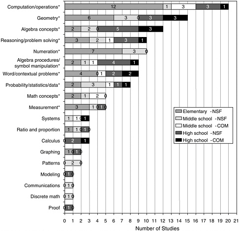
FIGURE 5-11 Study counts for all content strands.

tary curricula where no data were available) in the forms of percentages, with the frequencies listed in the bars.

The presentation of results by strands must be accompanied by the same restrictions as stated previously. These results are based on studies identified as at least minimally methodologically adequate. The quality of the outcome measures in measuring the content strands has not been examined. Their results are coded in relation to the comparison group in the study and are indicated as statistically in favor of the program, as in favor of the comparative program, or as showing no significant differences. The results are combined across studies with no weighting by study size. Their results should be viewed as a means for the identification of topics for potential future study. It is completely possible that a refinement of methodologies may affect the future patterns of results, so the results are to be viewed as tentative and suggestive.

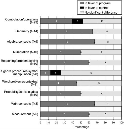
FIGURE 5-12 Major content strand result: All NSF (n=27).

According to these tentative results, future evaluations should examine whether the NSF-supported programs produce sufficient competency among students in the areas of algebraic manipulation and computation. In computation, approximately 40 percent of the results were in favor of the treatment group, no significant differences were reported in approximately 50 percent of the results, and results in favor of the comparison were revealed 10 percent of the time. Interpreting that final proportion of no significant difference is essential. Some would argue that because computation has not been emphasized, findings of no significant differences are acceptable. Others would suggest that such findings indicate weakness, because the development of the materials and accompanying professional development yielded no significant difference in key areas.

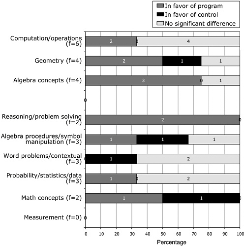
FIGURE 5-13 Major content strand result: All commercial (n=8).

From Figure 5-13 of findings from studies of commercially generated curricula, it appears that mixed results are commonly reported. Thus, in evaluations of commercial materials, lack of significant differences in computations/operations, word problems, and probability and statistics suggest that careful attention should be given to measuring these outcomes in future evaluations.

Overall, the grade band results for the NSF-supported programs—while consistent with the aggregated results—provide more detail. At the elementary level, evaluations of NSF-supported curricula (n=12) report better performance in mathematics concepts, geometry, and reasoning and problem solving, and some weaknesses in computation. No content strand analysis for commercially generated materials was possible. Evaluations

(n=6) at middle grades of NSF-supported curricula showed strength in measurement, geometry, and probability and statistics and some weaknesses in computation. In the studies of commercial materials, evaluations (n=4) reported favorable results in reasoning and problem solving and some unfavorable results in algebraic procedures, contextual problems, and mathematics concepts. Finally, at the high school level, the evaluations (n=9) by content strand for the NSF-supported curricula showed strong favorable results in algebra concepts, reasoning/problem solving, word problems, probability and statistics, and measurement. Results in favor of the control were reported in 25 percent of the algebra procedures and 33 percent of computation measures.

For the studies of commercial materials (n=4), only the geometry results favor the control group 25 percent of the time, with 50 percent having favorable results. Algebra concepts, reasoning, and probability and statistics also produced favorable results.

Equity Analysis of Comparative Studies

When the goal of providing a standards-based curriculum to all students was proposed, most people could recognize its merits: the replacement of dull, repetitive, largely dead-end courses with courses that would lead all students to be able, if desired and earned, to pursue careers in mathematics-reliant fields. It was clear that the NSF-supported projects, a stated goal of which was to provide standards-based courses to all students, called for curricula that would address the problem of too few students persisting in the study of mathematics. For example, as stated in the NSF Request for Proposals (RFP):

Rather than prematurely tracking students by curricular objectives, secondary school mathematics should provide for all students a common core of mainstream mathematics differentiated instructionally by level of abstraction and formalism, depth of treatment and pace (National Science Foundation, 1991, p. 1). In the elementary level solicitation, a similar statement on causes for all students was made (National Science Foundation, 1988, pp. 4-5).

Some, but not enough attention has been paid to the education of students who fall below the average of the class. On the other hand, because the above average students sometimes do not receive a demanding education, it may be incorrectly assumed they are easy to teach (National Science Foundation, 1989, p. 2).

Likewise, with increasing numbers of students in urban schools, and increased demographic diversity, the challenges of equity are equally significant for commercial publishers, who feel increasing pressures to demonstrate the effectiveness of their products in various contexts.

The problem was clearly identified: poorer performance by certain subgroups of students (minorities—non-Asian, LEP students, sometimes females) and a resulting lack of representation of such groups in mathematics-reliant fields. In addition, a secondary problem was acknowledged: Highly talented American students were not being provided adequate challenge and stimulation in comparison with their international counterparts. We relied on the concept of equity in examining the evaluation. Equity was contrasted to equality, where one assumed all students should be treated exactly the same (Secada et al., 1995). Equity was defined as providing opportunities and eliminating barriers so that the membership in a subgroup does not subject one to undue and systematically diminished possibility of success in pursuing mathematical study. Appropriate treatment therefore varies according to the needs of and obstacles facing any subgroup.

Applying the principles of equity to evaluate the progress of curricular programs is a conceptually thorny challenge. What is challenging is how to evaluate curricular programs on their progress toward equity in meeting the needs of a diverse student body. Consider how the following questions provide one with a variety of perspectives on the effectiveness of curricular reform regarding equity:

Does one expect all students to improve performance, thus raising the bar, but possibly not to decrease the gap between traditionally well-served and under-served students?

Does one focus on reducing the gap and devote less attention to overall gains, thus closing the gap but possibly not raising the bar?

Or, does one seek evidence that progress is made on both challenges—seeking progress for all students and arguably faster progress for those most at risk?

Evaluating each of the first two questions independently seems relatively straightforward. When one opts for a combination of these two, the potential for tensions between the two becomes more evident. For example, how can one differentiate between the case in which the gap is closed because talented students are being underchallenged from the case in which the gap is closed because the low-performing students improved their progress at an increased rate? Many believe that nearly all mathematics curricula in this country are insufficiently challenging and rigorous. Therefore achieving modest gains across all ability levels with evidence of accelerated progress by at-risk students may still be criticized for failure to stimulate the top performing student group adequately. Evaluating curricula with regard to this aspect therefore requires judgment and careful methodological attention.

Depending on one’s view of equity, different implications for the collection of data follow. These considerations made examination of the quality of the evaluations as they treated questions of equity challenging for the committee members. Hence we spell out our assumptions as precisely as possible:

Evaluation studies should include representative samples of student demographics, which may require particular attention to the inclusion of underrepresented minority students from lower socioeconomic groups, females, and special needs populations (LEP, learning disabled, gifted and talented students) in the samples. This may require one to solicit participation by particular schools or districts, rather than to follow the patterns of commercial implementation, which may lead to an unrepresentative sample in aggregate.

Analysis of results should always consider the impact of the program on the entire spectrum of the sample to determine whether the overall gains are distributed fairly among differing student groups, and not achieved as improvements in the mean(s) of an identifiable subpopulation(s) alone.

Analysis should examine whether any group of students is systematically less well served by curricular implementation, causing losses or weakening the rate of gains. For example, this could occur if one neglected the continued development of programs for gifted and talented students in mathematics in order to implement programs focused on improving access for underserved youth, or if one improved programs solely for one group of language learners, ignoring the needs of others, or if one’s study systematically failed to report high attrition affecting rates of participation of success or failure.

Analyses should examine whether gaps in scores between significantly disadvantaged or underperforming subgroups and advantaged subgroups are decreasing both in relation to eliminating the development of gaps in the first place and in relation to accelerating improvement for underserved youth relative to their advantaged peers at the upper grades.

In reviewing the outcomes of the studies, the committee reports first on what kinds of attention to these issues were apparent in the database, and second on what kinds of results were produced. Some of the studies used multiple methods to provide readers with information on these issues. In our report on the evaluations, we both provide descriptive information on the approaches used and summarize the results of those studies. Developing more effective methods to monitor the achievement of these objectives may need to go beyond what is reported in this study.

Among the 63 at least minimally methodologically adequate studies, 26 reported on the effects of their programs on subgroups of students. The

TABLE 5-13 Most Common Subgroups Used in the Analyses and the Number of Studies That Reported on That Variable

other 37 reported on the effects of the curricular intervention on means of whole groups and their standard deviations, but did not report on their data in terms of the impact on subpopulations. Of those 26 evaluations, 19 studies were on NSF-supported programs and 7 were on commercially generated materials. Table 5-13 reports the most common subgroups used in the analyses and the number of studies that reported on that variable. Because many studies used multiple categories for disaggregation (ethnicity, SES, and gender), the number of reports is more than double the number of studies. For this reason, we report the study results in terms of the “frequency of reports on a particular subgroup” and distinguish this from what we refer to as “study counts.” The advantage of this approach is that it permits reporting on studies that investigated multiple ways to disaggregate their data. The disadvantage is that in a sense, studies undertaking multiple disaggregations become overrepresented in the data set as a result. A similar distinction and approach were used in our treatment of disaggregation by content strands.

It is apparent from these data that the evaluators of NSF-supported curricula documented more equity-based outcomes, as they reported 43 of the 56 comparisons. However, the same percentage of the NSF-supported evaluations disaggregated their results by subgroup, as did commercially generated evaluations (41 percent in both cases). This is an area where evaluations of curricula could benefit greatly from standardization of ex-

pectation and methodology. Given the importance of the topic of equity, it should be standard practice to include such analyses in evaluation studies.

In summarizing these 26 studies, the first consideration was whether representative samples of students were evaluated. As we have learned from medical studies, if conclusions on effectiveness are drawn without careful attention to representativeness of the sample relative to the whole population, then the generalizations drawn from the results can be seriously flawed. In Chapter 2 we reported that across the studies, approximately 81 percent of the comparative studies and 73 percent of the case studies reported data on school location (urban, suburban, rural, or state/region), with suburban students being the largest percentage in both study types. The proportions of students studied indicated a tendency to undersample urban and rural populations and oversample suburban schools. With a high concentration of minorities and lower SES students in these areas, there are some concerns about the representativeness of the work.

A second consideration was to see whether the achievement effects of curricular interventions were achieved evenly among the various subgroups. Studies answered this question in different ways. Most commonly, evaluators reported on the performance of various subgroups in the treatment conditions as compared to those same subgroups in the comparative condition. They reported outcome scores or gains from pretest to posttest. We refer to these as “between” comparisons.

Other studies reported on the differences among subgroups within an experimental treatment, describing how well one group does in comparison with another group. Again, these reports were done in relation either to outcome measures or to gains from pretest to posttest. Often these reports contained a time element, reporting on how the internal achievement patterns changed over time as a curricular program was used. We refer to these as “within” comparisons.

Some studies reported both between and within comparisons. Others did not report findings by comparing mean scores or gains, but rather created regression equations that predicted the outcomes and examined whether demographic characteristics are related to performance. Six studies (all on NSF-supported curricula) used this approach with variables related to subpopulations. Twelve studies used ANCOVA or Multiple Analysis of Variance (MANOVA) to study disaggregation by subgroup, and two reported on comparative effect sizes. In the studies using statistical tests other than t-tests or Chi-squares, two were evaluations of commercially generated materials and the rest were of NSF-supported materials.

Of the studies that reported on gender (n=19), the NSF-supported ones (n=13) reported five cases in which the females outperformed their counterparts in the controls and one case in which the female-male gap decreased within the experimental treatments across grades. In most cases, the studies

present a mixed picture with some bright spots, with the majority showing no significant difference. One study reported significant improvements for African-American females.

In relation to race, 15 of 16 reports on African Americans showed positive effects in favor of the treatment group for NSF-supported curricula. Two studies reported decreases in the gaps between African Americans and whites or Asians. One of the two evaluations of African Americans, performance reported for the commercially generated materials, showed significant positive results, as mentioned previously.

For Hispanic students, 12 of 15 reports of the NSF-supported materials were significantly positive, with the other 3 showing no significant difference. One study reported a decrease in the gaps in favor of the experimental group. No evaluations of commercially generated materials were reported on Hispanic populations. Other reports on ethnic groups occurred too seldom to generalize.

Students from lower socioeconomic groups fared well, according to reported evaluations of NSF-supported materials (n=8), in that experimental groups outperformed control groups in all but one case. The one study of commercially generated materials that included SES as a variable reported no significant difference. For students with limited English proficiency, of the two evaluations of NSF-supported materials, one reported significantly more positive results for the experimental treatment. Likewise, one study of commercially generated materials yielded a positive result at the elementary level.

We also examined the data for ability differences and found reports by quartiles for a few evaluation studies. In these cases, the evaluations showed results across quartiles in favor of the NSF-supported materials. In one case using the same program, the lower quartiles showed the most improvement, and in the other, the gains were in the middle and upper groups for the Iowa Test of Basic Skills and evenly distributed for the informal assessment.

Summary Statements

After reviewing these studies, the committee observed that examining differences by gender, race, SES, and performance levels should be examined as a regular part of any review of effectiveness. We would recommend that all comparative studies report on both “between” and “within” comparisons so that the audience of an evaluation can simply and easily consider the level of improvement, its distribution across subgroups, and the impact of curricular implementation on any gaps in performance. Each of the major categories—gender, race/ethnicity, SES, and achievement level—contributes a significant and contrasting view of curricular impact. Further-

more, more sophisticated accounts would begin to permit, across studies, finer distinctions to emerge, such as the effect of a program on young African-American women or on first generation Asian students.

In addition, the committee encourages further study and deliberation on the use of more complex approaches to the examination of equity issues. This is particularly important due to the overlaps among these categories, where poverty can show itself as its own variable but also may be highly correlated to prior performance. Hence, the use of one variable can mask differences that should be more directly attributable to another. The committee recommends that a group of measurement and equity specialists confer on the most effective design to advance on these questions.

Finally, it is imperative that evaluation studies systematically include demographically representative student populations and distinguish evaluations that follow the commercial patterns of use from those that seek to establish effectiveness with a diverse student population. Along these lines, it is also important that studies report on the impact data on all substantial ethnic groups, including whites. Many studies, perhaps because whites were the majority population, failed to report on this ethnic group in their analyses. As we saw in one study, where Asian students were from poor homes and first generation, any subgroup can be an at-risk population in some setting, and because gains in means may not necessarily be assumed to translate to gains for all subgroups or necessarily for the majority subgroup. More complete and thorough descriptions and configurations of characteristics of the subgroups being served at any location—with careful attention to interactions—is needed in evaluations.

Interactions Among Content and Equity, by Grade Band

By examining disaggregation by content strand by grade levels, along with disaggregation by diverse subpopulations, the committee began to discover grade band patterns of performance that should be useful in the conduct of future evaluations. Examining each of these issues in isolation can mask some of the overall effects of curricular use. Two examples of such analysis are provided. The first example examines all the evaluations of NSF-supported curricula from the elementary level. The second examines the set of evaluations of NSF-supported curricula at the high school level, and cannot be carried out on evaluations of commercially generated programs because they lack disaggregation by student subgroup.

Example One

At the elementary level, the findings of the review of evaluations of data on effectiveness of NSF-supported curricula report consistent patterns of

benefits to students. Across the studies, it appears that positive results are enhanced when accompanied by adequate professional development and the use of pedagogical methods consistent with those indicated by the curricula. The benefits are most consistently evidenced in the broadening topics of geometry, measurement, probability, and statistics, and in applied problem solving and reasoning. It is important to consider whether the outcome measures in these areas demonstrate a depth of understanding. In early understanding of fractions and algebra, there is some evidence of improvement. Weaknesses are sometimes reported in the areas of computational skills, especially in the routinization of multiplication and division. These assertions are tentative due to the possible flaws in designs but quite consistent across studies, and future evaluations should seek to replicate, modify, or discredit these results.

The way to most efficiently and effectively link informal reasoning and formal algorithms and procedures is an open question. Further research is needed to determine how to most effectively link the gains and flexibility associated with student-generated reasoning to the automaticity and generalizability often associated with mastery of standard algorithms.

The data from these evaluations at the elementary level generally present credible evidence of increased success in engaging minority students and students in poverty based on reported gains that are modestly higher for these students than for the comparative groups. What is less well documented in the studies is the extent to which the curricula counteract the tendencies to see gaps emerge and result in long-term persistence in performance by gender and minority group membership as they move up the grades. However, the evaluations do indicate that these curricula can help, and almost never do harm. Finally, on the question of adequate challenge for advanced and talented students, the data are equivocal. More attention to this issue is needed.

Example Two

The data at the high school level produced the most conflicting results, and in conducting future evaluations, evaluators will need to examine this level more closely. We identify the high school as the crucible for curricular change for three reasons: (1) the transition to postsecondary education puts considerable pressure on these curricula; (2) the criteria outlined in the NSF RFP specify significant changes from traditional practice; and (3) high school freshmen arrive from a myriad of middle school curricular experiences. For the NSF-supported curricula, the RFP required that the programs provide a core curriculum “drawn from statistics/probability, algebra/functions, geometry/trigonometry, and discrete mathematics” (NSF, 1991, p. 2) and use “a full range of tools, including graphing calculators

and computers” (NSF, 1991, p. 2). The NSF RFP also specified the inclusion of “situations from the natural and social sciences and from other parts of the school curriculum as contexts for developing and using mathematics” (NSF, 1991, p. 1). It was during the fourth year that “course options should focus on special mathematical needs of individual students, accommodating not only the curricular demands of the college-bound but also specialized applications supportive of the workplace aspirations of employment-bound students” (NSF, 1991, p. 2). Because this set of requirements comprises a significant departure from conventional practice, the implementation of the high school curricula should be studied in particular detail.

We report on a Systemic Initiative for Montana Mathematics and Science (SIMMS) study by Souhrada (2001) and Brown et al. (1990), in which students were permitted to select traditional, reform, and mixed tracks. It became apparent that the students were quite aware of the choices they faced, as illustrated in the following quote:

The advantage of the traditional courses is that you learn—just math. It’s not applied. You get a lot of math. You may not know where to use it, but you learn a lot…. An advantage in SIMMS is that the kids in SIMMS tell me that they really understand the math. They understand where it comes from and where it is used.

This quote succinctly captures the tensions reported as experienced by students. It suggests that student perceptions are an important source of evidence in conducting evaluations. As we examined these curricular evaluations across the grades, we paid particular attention to the specificity of the outcome measures in relation to curricular objectives. Overall, a review of these studies would lead one to draw the following tentative summary conclusions:

There is some evidence of discontinuity in the articulation between high school and college, resulting from the organization and emphasis of the new curricula. This discontinuity can emerge in scores on college admission tests, placement tests, and first semester grades where nonreform students have shown some advantage on typical college achievement measures.

The most significant areas of disadvantage seem to be in students’ facility with algebraic manipulation, and with formalization, mathematical structure, and proof when isolated from context and denied technological supports. There is some evidence of weakness in computation and numeration, perhaps due to reliance on calculators and varied policies regarding their use at colleges (Kahan, 1999; Huntley et al., 2000).

There is also consistent evidence that the new curricula present

strengths in areas of solving applied problems, the use of technology, new areas of content development such as probability and statistics and functions-based reasoning in the use of graphs, using data in tables, and producing equations to describe situations (Huntley et al., 2000; Hirsch and Schoen, 2002).

Despite early performance on standard outcome measures at the high school level showing equivalent or better performance by reform students (Austin et al., 1997; Merlino and Wolff, 2001), the common standardized outcome measures (Preliminary Scholastic Assessment Test [PSAT] scores or national tests) are too imprecise to determine with more specificity the comparisons between the NSF-supported and comparison approaches, while program-generated measures lack evidence of external validity and objectivity. There is an urgent need for a set of measures that would provide detailed information on specific concepts and conceptual development over time and may require use as embedded as well as summative assessment tools to provide precise enough data on curricular effectiveness.

The data also report some progress in strengthening the performance of underrepresented groups in mathematics relative to their counterparts in the comparative programs (Schoen et al., 1998; Hirsch and Schoen, 2002).

This reported pattern of results should be viewed as very tentative, as there are only a few studies in each of these areas, and most do not adequately control for competing factors, such as the nature of the course received in college. Difficulties in the transition may also be the result of a lack of alignment of measures, especially as placement exams often emphasize algebraic proficiencies. These results are presented only for the purpose of stimulating further evaluation efforts. They further emphasize the need to be certain that such designs examine the level of mathematical reasoning of students, particularly in relation to their knowledge of understanding of the role of proofs and definitions and their facility with algebraic manipulation as we as carefully document the competencies taught in the curricular materials. In our framework, gauging the ease of transition to college study is an issue of examining curricular alignment with systemic factors, and needs to be considered along with those tests that demonstrate a curricular validity of measures. Furthermore, the results raising concerns about college success need replication before secure conclusions are drawn.

Also, it is important that subsequent evaluations also examine curricular effects on students’ interest in mathematics and willingness to persist in its study. Walker (1999) reported that there may be some systematic differences in these behaviors among different curricula and that interest and persistence may help students across a variety of subgroups to survive entry-level hurdles, especially if technical facility with symbol manipulation

can be improved. In the context of declines in advanced study in mathematics by American students (Hawkins, 2003), evaluation of curricular impact on students’ interest, beliefs, persistence, and success are needed.

The committee takes the position that ultimately the question of the impact of different curricula on performance at the collegiate level should be resolved by whether students are adequately prepared to pursue careers in mathematical sciences, broadly defined, and to reason quantitatively about societal and technological issues. It would be a mistake to focus evaluation efforts solely or primarily on performance on entry-level courses, which can clearly function as filters and may overly emphasize procedural competence, but do not necessarily represent what concepts and skills lead to excellence and success in the field.

These tentative patterns of findings indicate that at the high school level, it is necessary to conduct individual evaluations that examine the transition to college carefully in order to gauge the level of success in preparing students for college entry and the successful negotiation of majors. Equally, it is imperative to examine the impact of high school curricula on other possible student trajectories, such as obtaining high school diplomas, moving into worlds of work or through transitional programs leading to technical training, two-year colleges, and so on.

These two analyses of programs by grade-level band, content strand, and equity represent a methodological innovation that could strengthen the empirical database on curricula significantly and provide the level of detail really needed by curriculum designers to improve their programs. In addition, it appears that one could characterize the NSF programs (and not the commercial programs as a group) as representing a particular approach to curriculum, as discussed in Chapter 3 . It is an approach that integrates content strands; relies heavily on the use of situations, applications, and modeling; encourages the use of technology; and has a significant dose of mathematical inquiry. One could ask the question of whether this approach as a whole is “effective.” It is beyond the charge and scope of this report, but is a worthy target of investigation if one uses proper care in design, execution, and analysis. Likewise other approaches to curricular change should be investigated at the aggregate level, using careful and rigorous design.

The committee believes that a diversity of curricular approaches is a strength in an educational system that maintains local and state control of curricular decision making. While “scientifically established as effective” should be an increasingly important consideration in curricular choice, local cultural differences, needs, values, and goals will also properly influence curricular choice. A diverse set of effective curricula would be ideal. Finally, the committee emphasizes once again the importance of basing the studies on measures with established curricular validity and avoiding cor-

ruption of indicators as a result of inappropriate amounts of teaching to the test, so as to be certain that the outcomes are the product of genuine student learning.

CONCLUSIONS FROM THE COMPARATIVE STUDIES

In summary, the committee reviewed a total of 95 comparative studies. There were more NSF-supported program evaluations than commercial ones, and the commercial ones were primarily on Saxon or UCSMP materials. Of the 19 curricular programs reviewed, 23 percent of the NSF-supported and 33 percent of the commercially generated materials selected had programs with no comparative reviews. This finding is particularly disturbing in light of the legislative mandate in No Child Left Behind (U.S. Department of Education, 2001) for scientifically based curricular programs and materials to be used in the schools. It suggests that more explicit protocols for the conduct of evaluation of programs that include comparative studies need to be required and utilized.

Sixty-nine percent of NSF-supported and 61 percent of commercially generated program evaluations met basic conditions to be classified as at least minimally methodologically adequate studies for the evaluation of effectiveness. These studies were ones that met the criteria of including measures of student outcomes on mathematical achievement, reporting a method of establishing comparability among samples and reporting on implementation elements, disaggregating by content strand, or using precise, theoretical analyses of the construct or multiple measures.

Most of these studies had both strengths and weaknesses in their quasi-experimental designs. The committee reviewed the studies and found that evaluators had developed a number of features that merit inclusions in future work. At the same time, many had internal threats to validity that suggest a need for clearer guidelines for the conduct of comparative evaluations.

Many of the strengths and innovations came from the evaluators’ understanding of the program theories behind the curricula, their knowledge of the complexity of practice, and their commitment to measuring valid and significant mathematical ideas. Many of the weaknesses came from inadequate attention to experimental design, insufficient evidence of the independence of evaluators in some studies, and instability and lack of cooperation in interfacing with the conditions of everyday practice.

The committee identified 10 elements of comparative studies needed to establish a basis for determining the effectiveness of a curriculum. We recognize that not all studies will be able to implement successfully all elements, and those experimental design variations will be based largely on study size and location. The list of elements begins with the seven elements

corresponding to the seven critical decisions and adds three additional elements that emerged as a result of our review:

A better balance needs to be achieved between experimental and quasi-experimental studies. The virtual absence of large-scale experimental studies does not provide a way to determine whether the use of quasi-experimental approaches is being systematically biased in unseen ways.

If a quasi-experimental design is selected, it is necessary to establish comparability. When quasi-experimentation is used, it “pertains to studies in which the model to describe effects of secondary variables is not known but assumed” (NRC, 1992, p. 18). This will lead to weaker and potentially suspect causal claims, which should be acknowledged in the evaluation report, but may be necessary in relation to feasibility (Joint Committee on Standards for Educational Evaluation, 1994). In general, to date, studies have assumed prior achievement measures, ethnicity, gender, and SES, are acceptable variables on which to match samples or on which to make statistical adjustments. But there are often other variables in need of such control in such evaluations including opportunity to learn, teacher effectiveness, and implementation (see #4 below).

The selection of a unit of analysis is of critical importance to the design. To the extent possible, it is useful to randomly assign the unit for the different curricula. The number of units of analysis necessary for the study to establish statistical significance depends not on the number of students, but on this unit of analysis. It appears that classrooms and schools are the most likely units of analysis. In addition, the development of increasingly sophisticated means of conducting studies that recognize that the level of the educational system in which experimentation occurs affects research designs.

It is essential to examine the implementation components through a set of variables that include the extent to which the materials are implemented, teaching methods, the use of supplemental materials, professional development resources, teacher background variables, and teacher effects. Gathering these data to gauge the level of implementation fidelity is essential for evaluators to ensure adequate implementation. Studies could also include nested designs to support analysis of variation by implementation components.

Outcome data should include a variety of measures of the highest quality. These measures should vary by question type (open ended, multiple choice), by type of test (international, national, local) and by relation of testing to everyday practice (formative, summative, high stakes), and ensure curricular validity of measures and assess curricular alignment with systemic factors. The use of comparisons among total tests, fair tests, and

conservative tests, as done in the evaluations of UCSMP, permits one to gain insight into teacher effects and to contrast test results by items included. Tests should also include content strands to aid disaggregation, at a level of major content strands (see Figure 5-11 ) and content-specific items relevant to the experimental curricula.

Statistical analysis should be conducted on the appropriate unit of analysis and should include more sophisticated methods of analysis such as ANOVA, ANCOVA, MACOVA, linear regression, and multiple regression analysis as appropriate.

Reports should include clear statements of the limitations to generalization of the study. These should include indications of limitations in populations sampled, sample size, unique population inclusions or exclusions, and levels of use or attrition. Data should also be disaggregated by gender, race/ethnicity, SES, and performance levels to permit readers to see comparative gains across subgroups both between and within studies.

It is useful to report effect sizes. It is also useful to present item-level data across treatment program and show when performances between the two groups are within the 10 percent confidence interval of each other. These two extremes document how crucial it is for curricula developers to garner both precise and generalizable information to inform their revisions.

Careful attention should also be given to the selection of samples of populations for participation. These samples should be representative of the populations to whom one wants to generalize the results. Studies should be clear if they are generalizing to groups who have already selected the materials (prior users) or to populations who might be interested in using the materials (demographically representative).

The control group should use an identified comparative curriculum or curricula to avoid comparisons to unstructured instruction.

In addition to these prototypical decisions to be made in the conduct of comparative studies, the committee suggests that it would be ideal for future studies to consider some of the overall effects of these curricula and to test more directly and rigorously some of the findings and alternative hypotheses. Toward this end, the committee reported the tentative findings of these studies by program type. Although these results are subject to revision, based on the potential weaknesses in design of many of the studies summarized, the form of analysis demonstrated in this chapter provides clear guidance about the kinds of knowledge claims and the level of detail that we need to be able to judge effectiveness. Until we are able to achieve an array of comparative studies that provide valid and reliable information on these issues, we will be vulnerable to decision making based excessively on opinion, limited experience, and preconceptions.

This book reviews the evaluation research literature that has accumulated around 19 K-12 mathematics curricula and breaks new ground in framing an ambitious and rigorous approach to curriculum evaluation that has relevance beyond mathematics. The committee that produced this book consisted of mathematicians, mathematics educators, and methodologists who began with the following charge:

• Evaluate the quality of the evaluations of the thirteen National Science Foundation (NSF)-supported and six commercially generated mathematics curriculum materials;
• Determine whether the available data are sufficient for evaluating the efficacy of these materials, and if not;
• Develop recommendations about the design of a project that could result in the generation of more reliable and valid data for evaluating such materials.

The committee collected, reviewed, and classified almost 700 studies, solicited expert testimony during two workshops, developed an evaluation framework, established dimensions/criteria for three methodologies (content analyses, comparative studies, and case studies), drew conclusions on the corpus of studies, and made recommendations for future research.

Welcome to OpenBook!

You're looking at OpenBook, NAP.edu's online reading room since 1999. Based on feedback from you, our users, we've made some improvements that make it easier than ever to read thousands of publications on our website.

Do you want to take a quick tour of the OpenBook's features?

Show this book's table of contents , where you can jump to any chapter by name.

...or use these buttons to go back to the previous chapter or skip to the next one.

Jump up to the previous page or down to the next one. Also, you can type in a page number and press Enter to go directly to that page in the book.

Switch between the Original Pages , where you can read the report as it appeared in print, and Text Pages for the web version, where you can highlight and search the text.

To search the entire text of this book, type in your search term here and press Enter .

Share a link to this book page on your preferred social network or via email.

View our suggested citation for this chapter.

Ready to take your reading offline? Click here to buy this book in print or download it as a free PDF, if available.

Get Email Updates

Do you enjoy reading reports from the Academies online for free ? Sign up for email notifications and we'll let you know about new publications in your areas of interest when they're released.

• Master Your Homework
• Do My Homework

Writing Reports and Research Papers: A Comparison

Writing reports and research papers are two of the most common forms of academic writing for students. However, these types of documents differ in purpose, structure and style. This article provides an overview of how to approach each type when composing a paper or report, highlighting their similarities as well as differences between them. In addition to outlining key points on structuring both reports and research papers according to accepted academic conventions, it also focuses on developing a meaningful understanding between the two genres that will help create coherent written documents with appropriate depth for different contexts. Furthermore, this analysis offers insight into ways one can combine elements from both styles in order to meet specific communicative needs effectively within any given project’s parameters.

I. Introduction

Ii. definition of a report and research paper, iii. similarities between reports and research papers, iv. differences between reports and research papers, v. structure of the two types of documents, vi. writing styles for reports and research papers, vii. conclusion.

As a form of academic writing, research papers and reports have their own distinctive features. Research papers focus on providing an analysis of the current literature in order to contribute new insight into existing knowledge. On the other hand, Reports are written for various purposes such as documenting investigation results or summarizing research findings from others.

• Research Paper : A research paper is typically longer than other forms of writing and contains evidence-based arguments backed up by reliable data sources. It should also include well-structured discussion sections based upon relevant theories that support your argument.
• Report : In contrast to a research paper, reports are generally shorter documents with less detailed content and limited theoretical discussion. They may be used for conveying information about specific phenomena related to business activities or experiments conducted during laboratory practice sessions.

What Are Reports and Research Papers? Reports and research papers are two distinct forms of written communication used in the academic realm. Although both can be utilized for providing information on a given subject, there are fundamental differences between the two that make them suitable for different purposes.

A report , typically structured in sections or chapters, is intended to present findings from an investigation into a specific issue. It may summarize data obtained through interviews or surveys, observations made at a certain event or location, results from laboratory experiments and much more. A report provides factual information about the topic under consideration and seeks to explain its significance without making judgements or recommendations.

Conversely, a research paper presents evidence gathered by an author during their own study of particular subject matter. Its purpose is not only to provide readers with data but also analyze it critically using various approaches such as comparison or argumentation; thereby forming conclusions about it which might suggest implications for future investigations. The content may originate partially (or wholly) from outside sources such as other works related to similar topics; however they must be appropriately referenced according too accepted standards like APA 6th Edition format .

Common Threads Reports and research papers have certain characteristics that tie them together. While reports are typically shorter than research papers, both include an introduction to the topic, a discussion of findings and ideas related to the topic, as well as a conclusion or summary section. Both documents also require thorough organization and use of sources for credibility purposes. In this way, they provide readers with an opportunity to learn more about their given subject in depth.

Distinct Characteristics However, there are still important differences between the two types of written work. Reports focus more on factual information while research papers delve deeper into analysis by synthesizing facts from multiple perspectives. Furthermore, reports usually involve fewer external sources than those used within academic writing like in a typical research paper assignment; instead relying heavily upon data collected internally such as through surveys or interviews conducted during the project process itself.

• Reports: fact-focused with few external sources.
• Research Papers: Analysis-driven using many outside sources.

In academic writing, reports and research papers have some distinct differences. Both types of documents require the same level of comprehensive evaluation; however, a report will present summaries in an organized fashion while a research paper is more analytical and requires further exploration.

• Writing Style : Reports use formal language to provide short overviews with objective accuracy. Research papers employ creative techniques that include critical analysis.
• Purpose : Reports offer factual information for decision-making purposes or to document existing conditions. Conversely, research papers address topics through evidence-based arguments.

Documents can come in many shapes and sizes. In the academic world, two of the most common types are research papers and reports. Both serve their purpose but have some distinct differences.

• A research paper is an analysis of a topic that includes thorough examination of evidence from various sources to make arguments.

Style Guide When writing a report or research paper, it is essential to keep in mind the style guide that you will be following. Depending on your field of study and area of interest, there are several possible style guides to follow, such as APA (American Psychological Association) and MLA (Modern Language Association). Be sure to familiarize yourself with whichever guide you will be using before beginning your project.

Research Paper vs Report It can often be difficult for students to understand the difference between a research paper and a report when both require similar levels of critical thinking skills. A research paper focuses more heavily on gathering evidence from different sources while drawing connections among various pieces of information gathered throughout the process; reports rely more heavily on facts already present without too much interpretation or analysis. Reports tend to take an objective stance when presenting data whereas papers may delve into deeper analysis regarding how certain phenomena interact with each other over time.

In summary, this project has highlighted the differences between research papers and reports. Research papers are longer, in-depth documents that involve academic research to uncover new knowledge or provide critical analysis of existing ideas. Reports are shorter summaries used to communicate information about a specific topic.

The two document types have different purposes but both require careful consideration when constructing them. When writing a research paper you must remain objective, while when creating a report it is acceptable to give your opinion as long as it is well supported with evidence from reliable sources. No matter what type of document you’re producing though, keep an eye on accuracy and clarity throughout.

English: The comparison between writing reports and research papers has been an ongoing discussion in academic circles for many years. This article provides a useful overview of the similarities and differences between these two types of writings, as well as considerations when deciding which approach to take. Ultimately, the best approach depends on the purpose of the document and the audience it will reach. Whether creating a report or research paper, understanding both approaches is essential to effective communication within academia.

Thank you for visiting nature.com. You are using a browser version with limited support for CSS. To obtain the best experience, we recommend you use a more up to date browser (or turn off compatibility mode in Internet Explorer). In the meantime, to ensure continued support, we are displaying the site without styles and JavaScript.

• View all journals
• My Account Login
• Explore content
• About the journal
• Publish with us
• Sign up for alerts
• Open access
• Published: 25 March 2024

Comparison of the effectiveness of different normalization methods for metagenomic cross-study phenotype prediction under heterogeneity

• Beibei Wang 1 , 2 , 3 ,
• Fengzhu Sun 4 &
• Yihui Luan 1 , 2 , 3  

Scientific Reports volume  14 , Article number:  7024 ( 2024 ) Cite this article

48 Accesses

1 Altmetric

Metrics details

• Computational biology and bioinformatics
• Machine learning

The human microbiome, comprising microorganisms residing within and on the human body, plays a crucial role in various physiological processes and has been linked to numerous diseases. To analyze microbiome data, it is essential to account for inherent heterogeneity and variability across samples. Normalization methods have been proposed to mitigate these variations and enhance comparability. However, the performance of these methods in predicting binary phenotypes remains understudied. This study systematically evaluates different normalization methods in microbiome data analysis and their impact on disease prediction. Our findings highlight the strengths and limitations of scaling, compositional data analysis, transformation, and batch correction methods. Scaling methods like TMM show consistent performance, while compositional data analysis methods exhibit mixed results. Transformation methods, such as Blom and NPN, demonstrate promise in capturing complex associations. Batch correction methods, including BMC and Limma, consistently outperform other approaches. However, the influence of normalization methods is constrained by population effects, disease effects, and batch effects. These results provide insights for selecting appropriate normalization approaches in microbiome research, improving predictive models, and advancing personalized medicine. Future research should explore larger and more diverse datasets and develop tailored normalization strategies for microbiome data analysis.

Similar content being viewed by others

Analysis of microbial compositions: a review of normalization and differential abundance analysis

Huang Lin & Shyamal Das Peddada

Multi-omic integration of microbiome data for identifying disease-associated modules

Efrat Muller, Itamar Shiryan & Elhanan Borenstein

Utilization of the microbiome in personalized medicine

Karina Ratiner, Dragos Ciocan, … Eran Elinav

Introduction

The human microbiome is a complex ecosystem of microorganisms that exist in symbiosis with the human body 1 . Extensive research has established that the human microbiome plays crucial roles in numerous physiological processes, including digestion, metabolism, immune system modulation, and even cognitive functions. Disruptions in the delicate microbial balance, known as dysbiosis, have been linked to a wide range of health conditions, including obesity 2 , 3 , diabetes 4 , inflammatory bowel disease 5 , 6 , allergies 7 , and several types of cancer 8 , 9 .

The advent of high-throughput sequencing technologies has revolutionized the field of microbiome research, enabling comprehensive profiling of microbial communities and providing insights into their roles in different physiological processes and disease states 10 . However, the analysis of microbiome data poses significant challenges due to inherent heterogeneity and variability across samples. Sources of variation can stem from technical differences in sequencing protocols 11 , variations in sample collection 12 and processing methods 13 , as well as biological diversity among individuals and populations. To extract meaningful insights from microbiome data, it is crucial to account for and mitigate these sources of variation.

Normalization methods have emerged as vital tools in addressing the heterogeneity and biases present in microbiome data. These methods aim to remove technical and biological biases, standardize data across samples, and enhance comparability between datasets. Various normalization approaches have been proposed, ranging from simple scaling methods to more advanced statistical techniques. Comparisons of normalization methods have been performed in the context of data distributions 14 , 15 and differential analysis 16 , 17 , 18 , 19 , 20 . Genotype-to-phenotype mapping is an essential problem in the current genomic era. In the realm of differential analysis and prediction, the application of normalization methods differs in their objectives. In differential analysis, the main objective of normalization among different datasets is to remove or mitigate spurious associations between microbes and diseases. On the other hand, the main objective of normalization for phenotype prediction is to increase prediction accuracy, robustness, reliability and generalizability of the trained model to the unseen testing data. However, the impact of normalization methods on phenotype predictions mainly focused on DNA microarray data and RNA-Seq data. Zwiener et al. 21 found rank-based transformations performed well in all scenarios in real RNA-Seq datasets. Franks et al. 22 proposed feature-wise quantile normalization (FSQN) and found FSQN successfully removes platform-based bias from RNA-Seq data, regardless of feature scaling or machine learning algorithm. Given the central role of normalization in microbiome data analysis and the lack of current methods comparison for microbiome data, there is a need to systematically evaluate their performance, particularly in the context of disease prediction.

In this paper, we provide a review of existing normalization methods and present a comprehensive evaluation of various normalization methods in predicting binary phenotypes using microbiome data. We examine the performance of scaling methods, compositional data analysis methods, transformation methods, and batch correction methods across simulated datasets and real datasets. Our analysis includes an assessment of prediction accuracy using metrics such as the area under the receiver operating characteristic curve (AUC), prediction accuracy, sensitivity, specificity, and the rank ordering of different methods.

By comparing and contrasting the performance of normalization methods across different datasets and phenotypic outcomes, we aim to provide insights into the strengths and limitations of each approach. This research will assist researchers and practitioners in selecting appropriate normalization methods for microbiome data analysis, thereby enhancing the robustness and reliability of predictive models in microbiome research.

Different datasets have different background distributions

There are eight publicly accessible colorectal cancer (CRC) datasets shown in Table 1 , including Feng 25 , Gupta 26 , 68 , Thomas 8 , Vogtmann 28 , Wirbel 29 , Yachida 30 , Yu 9 , and Zeller 31 . In total, we included 1260 samples (625 controls, 635 CRC cases) from multiple countries such as the USA, China, France, etc. The participant demographics ranged from 21 to 90 years, with a male representation of \(59.6\%\) . The datasets were characterized by diverse body mass index (BMI) values and included subjects with other health conditions such as hypertension, hypercholesterolemia, and Type 2 Diabetes (T2D). DNA extraction and sequencing were conducted using various protocols and platforms. Our analysis aimed to examine the background distribution differences among these datasets.

In order to assess population differences across the CRC datasets, a PCoA plot based on Bray Curtis distance was generated. Figure 1 a revealed distinct separations between different datasets, suggesting variations in microbial composition among the populations. Although the observed separation accounted for a small proportion ( \(7.9\%\) ) of the total variance, statistical significance was confirmed through the PERMANOVA test ( \(p=0.001\) ). These findings underscored the substantial heterogeneity in microbial communities across diverse CRC datasets, despite the relatively modest contribution to the overall variance. To quantify the overlaps of these datasets, we computed the average Bray-Curtis distance (Fig. 1 b). The dispersion of individual datasets was represented on the diagonal, with the largest dispersion observed in the Gupta dataset. Among the off-diagonal values that measured the average distance between samples in different datasets, Feng and Gupta exhibited the lowest overlap, with a distance of 0.901. Consequently, controls from these two datasets were selected as the template data for subsequent simulations in scenario 1. Mixing these two populations with decided proportions allowed us to control the heterogeneities between simulated populations.

Different CRC populations had different background distribution patterns. ( a ) PCoA plot based on Bray-Curtis distance, with colors for different datasets. The variance explained by populations (PERMANOVA \(R^2\) ) and its significance (PERMANOVA p value) were annotated in the figure. ( b ) Average Bray-Curtis distances between pairs of CRC datasets. Values on the diagonal referred to average Bray-Curtis distances between samples within the same dataset. Off-diagonal values refer to average Bray-Curtis distances between pairs of samples in different datasets. Larger values indicated a more dispersed distribution (on-diagonal) or bigger differences (off-diagonal). The figures were generated using R version 4.3.0.

Our analysis also extended to five distinct IBD datasets, as depicted in supplementary Table S1 . These included the Hall 32 , HMP 5 , 70 , Ijaz 33 , Nielsen 35 , and Vila 6 datasets. Similar to the CRC datasets, the IBD datasets exhibited variations in geographical origin, age, BMI, and sequencing platforms. Supplementary Figure S1 revealed a clear separation between the different datasets (Supplementary Figure S1 ( a )) along with evident dataset dispersion variations (Supplementary Figure S1 ( b )). These observations underscore the fact that distinctive populations are inherently marked by their unique background distributions, a factor that must be judiciously accounted for in any microbiome-related analysis.

Transformation and batch correction methods could enhance prediction performance for heterogeneous populations

In Scenario 1, the effects of different normalization methods on the prediction of binary phenotypes across diverse background distributions of taxa were investigated. The figures, including Figure 2 , Supplementary Figures S2 , S3 , and S4 , display the average performance metrics of 100 iterations: average AUC, accuracy, specificity, and sensitivity. Each panel in these figures represents a distinct disease effect, with each column denoting a population effect and rows indicating normalization methods.

Heatmaps depicting average AUC values obtained from abundance profiles normalized by various methods for predicting simulated cases and controls in Scenario 1. The panels ( a ), ( b ), and ( c ) correspond to disease effects of 1.02, 1.04, and 1.06 respectively. The columns represent different values of population effects, while the rows represent different normalization methods, grouped based on their classifications in the left column. The figures were generated using R version 4.3.0.

When there were no population effects between the training and testing datasets ( \(ep=0\) ), all normalization methods exhibited satisfactory performance, with average AUC, accuracy, sensitivity, and specificity values consistently achieving the maximum value of 1. However, as the population effects increased or disease effects decreased, an evident decline in these values was observed.

When the differences between case and control were small (Figure 2 ( a ), \(ed=1.02\) ), the prediction AUC values of scaling methods rapidly declined to 0.5 (random prediction value) as ep increased. TMM and RLE demonstrated better performances than TSS-based methods, such as UQ, MED, and CSS, in a wider range of conditions. Notably, TMM maintained an AUC value above 0.6 when \(ep<0.2\) . As disease effects increased (Figure 2 ( b ) \(ed=1.04\) and ( c ) \(ed=1.06\) ), both TMM and RLE exhibited superior ability to remove sample differences for predictions compared to TSS-based methods. Regarding prediction accuracy, TMM sustained accuracy above 0.6 with \(ed>1.04\) and \(ep<0.1\) , surpassing the accuracy of other techniques (Supplementary Figure S2 ). In comparison to TMM, the other normalization methods specifically designed for RNA-Seq data, such as RLE, showed a tendency to misclassify controls as cases in predictions. This resulted in a sensitivity close to 1 (Supplementary Figure S3 ) and a specificity close to 0 (Supplementary Figure S4 ) in scenarios with population effects between training and testing datasets ( \(ep>0\) ). Similar outcomes were observed for TSS but not for TSS-based methods such as UQ, MED, and CSS.

While normalized counts are commonly used for analyzing microbiome data, they still exhibit skewed distributions, unequal variances, and extreme values, which may limit their effectiveness in situations with significant heterogeneity. To enhance cross-population prediction performance, we applied various commonly used transformations, including CLR, LOG, AST, STD, Rank, Blom, NPN, logCPM, and VST. These transformation methods aimed to address one or several problems. For instance, logCPM and LOG transformations resolved skewness and extreme values, STD focused on unequal variances, VST tackled unequal variances and extreme values, and AST, CLR, Rank, Blom, and NPN addressed all three issues. The yellow and grey bars in Figure 2 represent the average prediction AUC values obtained using abundance profiles transformed by different methods. LOG, AST, Rank, and logCPM showed performances similar to TSS, indicating a failure in distribution adjustment. Conversely, transformation methods that achieved data normality, such as Blom and NPN, effectively aligned the data distributions across different populations for both population effects ( ep ) and disease effects ( ed ). Additionally, STD generally improved prediction AUC values, while the performance of CLR and VST transformation decreased with increasing population effects ( ep ). However, the sensitivity of all transformation methods was close to 1 (Supplementary Figure S3 ), and the specificity was close to 0 (Supplementary Figure S4 ) in circumstances where \(ep>0\) . Consequently, prediction accuracies remained around 0.5 (Supplementary Figure S2 ), even for methods like Blom, NPN, and STD that exhibited higher AUC values.

Surprisingly, the batch correction methods highlighted in red bars yielded promising prediction results with high AUC (Figure 2 ), accuracy (Supplementary Figure S3 ), sensitivity (Supplementary Figure S4 ), and specificity (Supplementary Figure S5 ), except for QN. QN forced the distribution of each sample to be the same, potentially distorting the true biological variation between case and control samples, making it difficult for the classifier to distinguish between the groups. This was also validated by its high sensitivity (Supplementary Figure S3 ) and low specificity (Supplementary Figure S4 ) values. While QN was only effective when the two populations originated from the same distribution, FSQN, BMC, limma, ComBat, and ConQuR significantly enhanced the reproducibility of response predictions, remaining unaffected by disease effects and population effects.

Batch correction methods can successfully remove batch effects within the same population

In Scenario 2, we examined studies within the same population that exhibited technical variations and differences across batches. These batch effects can lead to substantial heterogeneity among the data batches 71 . Figures 3 , S5, S6, and S7, respectively, showed the average AUC, accuracy, sensitivity, and specificity values obtained from random forest models using abundance profiles normalized by various methods across 100 runs. Overall, all these values demonstrated an upward trend with increasing disease effects. However, the normalization methods exhibited varying responses to changes in batch means and variances.

Figure 3 a displayed the results obtained with disease effect equal to 1.02. When the batch variance remained fixed ( \(sev_{var}=1\) ), pronounced response to additive batch means ( \(sev_{mean}=0,500,1000\) ) was observed among the scaling methods and some transformation methods (CLR, LOG, AST, logCPM, VST). These methods exhibited a decrease in AUC scores from approximately 0.7 to around 0.5 when \(sev_{mean}\ne 0\) . In contrast, the STD, Rank, Blom, NPN, and all batch correction methods maintained a more robust level of AUC values (around 0.7) in the presence of varying batch means, as long as the batch variances did not change. These trends persisted with increasing disease effects, as depicted in Fig. 3 b, c. Notably, among the methods more sensitive to batch means, scaling methods such as TMM and RLE exhibited a slight improvement in predictive accuracy as the batch means increased. Transformation methods like LOG, AST, and logCPM performed similarly.

The effects of batch variances on binary phenotype prediction remained consistent across different normalization methods. In Fig. 3 a, when the batch mean was fixed at 0 and the batch variances were adjusted from 1 to 4, all normalization methods experienced an average decrease in AUC values of approximately 0.1. Among the scaling methods, namely MED, UQ, and CSS, which modified the scaling factor from TSS, consistently yielded lower AUC values compared to other methods for different batch variances ( \(sev_{var}=1,2,4\) ). In Fig. 3 c, with \(ed=1.06\) , the influence of increased batch variance on prediction accuracy was reduced, indicating the dominance of disease effect in prediction. Most normalization methods achieved AUC scores above 0.9 when \(sev_{var}=4\) , indicating successful removal of batch effects for predictions. Nonetheless, MED, UQ, and CSS continued to exhibit inferior ability in removing batch effects compared to other methods.

In scenario 2, the general trends of prediction accuracy (Supplementary Figure S5 ), sensitivity (Supplementary Figure S6 ), and specificity (Supplementary Figure S7 ) aligned with AUC values. It is noteworthy that ComBat maintained prediction accuracy, sensitivity, and specificity at a lower level than other batch correction methods when the batch variance remained constant and the batch mean increased, highlighting its limitations in addressing batch mean discrepancies.

Heatmaps depicting average AUC values obtained from abundance profiles normalized by various methods for predicting simulated cases and controls in Scenario 2. The panels ( a ), ( b ), and ( c ) correspond to disease effects of 1.02, 1.04, and 1.06 respectively. The columns represent different combinations of batch mean and batch variation, with “m” for batch mean adjusting the mean and “v” for batch variance adjusting the variance. The rows represent different normalization methods, grouped based on their classifications in the left column. The figures were generated using R version 4.3.0.

The impact of disease model can be reduced by disease effects

In Scenario 3, we explored the influence of differences in disease models between the training and testing data on the prediction AUC scores. The results are presented in Figures 4 , S8, S9, and S10. The overall trends in the relative performance of different normalization methods were consistent with the previous two scenarios. The AUC scores increased as the disease effects increased. And as expected, the AUC scores also increased as the number of overlapping disease-related taxa increased. For example, when \(ed=1.02\) (Fig. 4 a), the AUC values obtained using abundance profiles normalized by different methods were all approximately 0.6 when there were 2 overlapping disease-associated taxa between the training and testing data. When the number of disease-associated taxa increased to 10, the optimal AUC scores increased to 0.7. The same pattern was observed with \(ed=1.04\) and \(ed=1.06\) . When the disease effects increased to 1.06 (Fig. 4 c), the majority of normalization methods achieved AUC scores exceeding 0.8, even when there were only 2 overlapped disease-associated taxa. This indicates that the impact of the disease model can be mitigated by stronger disease effects.

Figure 4 also illustrated that among the normalization methods we compared, scaling methods such as UQ, MED, and CSS had lower AUC values compared to other methods, as observed in the other two scenarios. QN also exhibited lower prediction performances. The other methods showed similar prediction performances with respect to different disease effects and different numbers of disease-associated taxa.

Supplementary Figures S8 , S9 , and S10 demonstrated a similar prediction performance of normalization methods measured by accuracy, sensitivity, and specificity.

Heatmaps depicting average AUC values obtained from abundance profiles normalized by various methods for predicting simulated cases and controls in Scenario 3. The panels ( a ), ( b ), and ( c ) correspond to disease effects of 1.02, 1.04, and 1.06 respectively. The columns represent different numbers of overlapping disease-associated taxa in the training and testing datasets. The rows represent different normalization methods, grouped based on their classifications in the left column. The figures were generated using R version 4.3.0.

Batch correction methods are necessary for cross-dataset predictions

We next evaluate various normalization methods using 8 gut microbiome datasets from shotgun sequencing related to CRC (Table 1 ). These experimental datasets were retrieved from the R package curatedMetagenomicData with a sample size larger than 30 for either cases or controls. Datasets were paired with one for model training and the other for validation. For each method, the AUC score, accuracy, sensitivity, and specificity based on the normalized abundance using random forest was calculated. We repeated the predictions 30 times to account for the randomness of the prediction model and the average of the these values was reported for each study.

Supplementary Figure S11 presents box plots showing the AUC values obtained from the 30 repeated predictions. We observed unstable AUC values for most normalization methods when trained or tested on the Gupta dataset. This observation aligns with the data distribution depicted in Fig. 1 , where Gupta exhibited the greatest dissimilarities and variability compared to other datasets. The same observation holds true for the Feng dataset. Overall, none of the normalization methods consistently improved the prediction AUC values to a specific level. The prediction accuracy remained dependent on both biological and technical factors. For example, when the model was trained on Gupta and tested on Feng, most methods yielded average AUC scores around 0.7, except for Rank and VST (Supplementary Figure S11 ( b1 )). None of the normalization methods achieved an AUC value above 0.8 to significantly improve prediction performance.

Distribution of ranks for 22 normalization methods in cross-dataset prediction on CRC datasets. The normalization methods are ranked based on the average AUC ( a ), average accuracy ( b ), average sensitivity ( c ), and average specificity ( d ) under the same pair of training and testing datasets. The figures were generated using R version 4.3.0.

The box plots of prediction accuracy, sensitivity, and specificity (Supplementary Figures S12 , S13 , and S14 ) are consistent with the results of AUC values, indicating that prediction outcomes are influenced by multiple factors, and normalization methods cannot fundamentally address the impact of heterogeneity on prediction reproducibility. Additionally, consistent with our observations in simulations, most methods exhibit a trend of high sensitivity and low specificity, suggesting that healthy individuals may be classified as diseased in clinical applications, requiring additional information for further assessment.

To quantify the performance of normalization methods, we ranked all normalization methods according to their average AUC, accuracy, sensitivity, and specificity values derived from models trained and tested on the same pair of training and testing datasets. The distributions of their ranks for each method are depicted in Figure 5 . A higher ranking (lower values in the box plot) indicates a better prediction performance. Among the twenty-two normalization methods we compared, batch correction methods, including FSQN, BMC, and Limma, tended to have higher AUC values (Figure 5 a) and higher accuracy (Figure 5 b) than other methods. In comparison to FSQN, BMC and Limma exhibited a superior balance between sensitivity and specificity. Most transformation methods encountered an issue of high sensitivity but low specificity, particularly evident in STD, Rank, and QN (Fig. 5 c, d). Scaling methods ranked behind batch correction methods and performed similarly to each other in CRC dataset predictions, indicating relatively small population effects in CRC datasets.

We also applied the normalization methods to IBD datasets listed in Supplementary Table S1 and conducted cross-dataset predictions. Supplementary Figures S15 , S16 , S17 , and S18 illustrates the box plots of the AUC, accuracy, sensitivity, and specificity values obtained from 30 repeated predictions, respectively. And Supplementary Figure S19 visualizes the rank distributions for each method within pairs of IBD datasets. The results obtained were similar to those observed in the CRC dataset predictions. Among all the normalization methods, batch correction methods, including BMC and Limma, consistently demonstrated the best performance. Scaling methods, such as TMM, followed closely behind. However, FSQN exhibited variable performance, occasionally achieving good results while sometimes yielding poor results. Overall, the trends in IBD dataset predictions were consistent with the observations made in CRC dataset predictions.

In our study, we considered three sources of heterogeneity between datasets: population effects, batch effects, and disease models. Population effect refers to variations arising from differences in population characteristics, including environmental factors, geographical locations, diet, and other population-specific features. If there are marked differences in the microbiome composition between the training and testing datasets, the trained model may struggle to distinguish disease-related microbiome patterns from population-specific variations. Batch effect arises from technical variations introduced during data collection or processing, such as sequencing technologies, sample preparation, or other experimental procedures. These batch effects may confound the true microbial signatures associated with the disease status, resulting in diminished generalization performance. Disease model represents the underlying patterns and features associated with the disease phenotype, and disparities in this regard can lead to decreased predictive performance, as a model trained on one dataset may encounter difficulties in generalizing effectively to another dataset. We conducted a comprehensive evaluation of various normalization methods for predicting binary phenotypes with the impact of heterogeneity from different sources. The results revealed important insights into the performance and suitability of different normalization approaches in the context of disease prediction.

Our findings demonstrated that no single normalization method consistently outperformed others across all datasets and phenotypic outcomes. This suggests that the choice of normalization method should be carefully considered based on the specific dataset characteristics and research objectives. However, certain trends and patterns did emerge from our analysis.

Among the scaling methods, methods such as TMM performed comparably well, indicating their effectiveness in reducing technical variations and improving the comparability of data across samples. These methods are relatively simple and straightforward to implement, making them practical choices for normalization in microbiome data analysis.

Interestingly, compositional data analysis methods, CLR, exhibited mixed performance across different datasets. While it has been widely used in microbial community analysis, our results suggest that its effectiveness in disease prediction may vary depending on the specific dataset and phenotypic outcome. Further investigation is needed to understand the underlying factors influencing the performance of compositional data analysis methods in predicting binary phenotypes.

Transformation methods, including NPN and Blom, showed promising results in some datasets according to the prediction AUC values, highlighting their potential to improve prediction performance by capturing nonlinear relationships and addressing skewed distributions. These methods offer flexibility in handling diverse data types and can be particularly valuable in situations where data transformation is necessary to meet model assumptions. However, trade-offs need to be made between prediction sensitivity and specificity when appluying transformation methods.

Batch correction methods, such as BMC and Limma, consistently performed well across multiple datasets. These methods effectively accounted for batch effects, which are often present in multi-center or multi-cohort studies. The ability to remove batch effects is critical in ensuring accurate and reliable predictions, especially when integrating data from different sources. Based on our findings, we recommend incorporating batch correction methods in cross-dataset binary phenotype prediction of metagenomic data. This involves utilizing scaling methods to mitigate biases attributed to sequencing technology, followed by LOG transformation to approximate a more normally distributed data, aligning with the assumptions of batch correction methods. By subsequently applying batch correction methods, we enhance the robustness of the analysis. We believe that this pipeline can improve the accuracy and reliability of phenotype cross-dataset predictions based on metagenomic data.

It is worth noting that the performance of normalization methods was influenced by the heterogeneity of the datasets. The relative impact of heterogeneity from different sources depends on the nature of the data and the extent of variation in each factor. For instance, if the population effect is pronounced and not adequately controlled, the model might capture population-specific differences instead of disease-related patterns. Likewise, if batch effects are left unaddressed, the model may overfit on technical variations instead of discerning true biological signals associated with the case-control status. In datasets where there were substantial biological and technical variations, the prediction accuracy remained primarily determined by these factors rather than the choice of normalization method. This emphasizes that proper preprocessing, normalization, and consideration of potential confounders are essential for building robust and generalizable predictive models.

Overall, our study underscores the need for careful consideration and evaluation of normalization methods in microbiome data analysis, particularly in the context of disease prediction. Researchers and practitioners should take into account the specific characteristics of their datasets, including population heterogeneity, disease effects, and technical variations when selecting and applying normalization methods. Additionally, future research should focus on developing novel normalization approaches that are tailored to the unique challenges of microbiome data and explore their performance in larger and more diverse datasets.

In conclusion, our comprehensive evaluation of normalization methods provides valuable insights into their performance in predicting binary phenotypes using microbiome data. This research contributes to the advancement of robust and reliable methodologies in microbiome research and paves the way for more accurate disease prediction and personalized therapeutic interventions based on the human microbiome.

Materials and methods

Real metagenomic dataests.

As the first application example, we analyzed shotgun sequencing data from patients with colorectal cancer (CRC) obtained from the R package curatedMetagenomicData v3.8.0 23 . The taxonomic profiles for each dataset were determined using MetaPhlAn3 24 , which ensures consistency in downstream analysis. A total of nine CRC datasets are available 8 , 9 , 25 , 26 , 27 , 28 , 29 , 30 , 31 . We excluded studies with sample sizes of less than 30 for either cases or controls, resulting in eight accessible CRC datasets for our analysis. A detailed summary outlining the distinctive characteristics of these eight CRC datasets can be found in Table 1 .

As the second application example, we analyzed shotgun sequencing data from patients with inflammatory bowel disease (IBD) from the R package curatedMetagenomicData v3.8.0 23 . There are 6 available IBD datasets in curatedMetagenomicData 5 , 6 , 32 , 33 , 34 , 35 . Similarly to the CRC datasets, we excluded studies with sample sizes less than 30 for either cases or controls from the analysis. A summary of the characteristics of the IBD datasets can be found in Supplementary Table S1 .

Statistical analysis

We calculated the microbial relative abundance for each sample and used the Bray-Curtis distance 36 to compare the dissimilarities between samples. This distance was computed using the function vegdist() from R package vegan 37 . To visualize the clustering of samples effectively, we performed principal coordinate analysis (PCoA) through the pcoa() function from R package ape 38 . To assess the variance attributable to datasets, we conducted the permutational multivariate analysis of variance (PERMANOVA) 39 with adonis() function in R package vegan 37 .

Normalization methods

A number of normalization methods could be applied to microbiome data for data analyses. For the purpose of predicting the unknown disease status of samples, we try to transform or normalize our data to satisfy the assumption that training and testing data are drawn from the same distribution. Seven scaling methods, one compositional data analysis method, eight transformation methods, and six batch correction methods were compared in this analysis. Our study is also the largest comparison in terms of prediction up to date according to our best knowledge.

Assume we have a dataset consisting of n samples and m features. Denote \(c_{ij}\) as the count for taxon i in sample j . With this notation, the steps and formula of normalization methods can be briefly introduced as follows.

Scaling methods

A commonly used method for normalizing microbiome data is scaling. Its basic idea is to divide counts in the taxa count table by a scaling factor or normalization factor to remove biases resulting from sequencing technology:

where \(x_{ij}\) is the normalized abundance for taxon i in sample j , \(s_j\) is the scaling/normalization factor for sample j . We investigated seven popular scaling methods (Table 2 ) in our analysis, including TSS, UQ, MED, CSS in metagenomeSeq , TMM in edgeR , RLE in DESeq2 , and GMPR in GUniFrac .

Total Sum Scaling (TSS) 14 : Counts are divided by the total number of reads in that sample.

Upper Quartile (UQ) 14 , 40 : Similar to TSS, it scales each sample by the upper quartile of counts different from 0 in that sample.

where \(q^3(\cdot )\) is the function of estimating upper quartile, and \(P_j=\{c_{ij}|c_{ij}>0, i=1,\cdots ,n\}\) represents a set of counts different from 0 in sample j .

Median (MED) 14 : Also similar to TSS, the total number of reads is replaced by the median counts different from 0 in the computation of the scaling factor.

where \(\text {Median}(\cdot )\) is the function of estimating median, and \(P_j=\{c_{ij}|c_{ij}>0, i=1,\cdots ,n\}\) represents a set of counts different from 0 in sample j .

Cumulative Sum Scaling (CSS) 41 : CSS modified TSS for microbiome data in a sample-specific manner. It selects the scaling factor as the cumulative sum of counts, up to a percentile \(\hat{l}\) determined by the data:

where \(M_j=\{c_{ij}|c_{ij}\le q_{\hat{l}}(c_{j})\}\) denotes the taxa included in the cumulative summation for sample j , and \(N^{\text {CSS}}\) is an appropriately chosen normalization constant. This scaling method is implemented by calling the cumNorm() function in the R package metagenomeSeq 41 .

Trimmed Mean of M-values (TMM) 42 : TMM is a popular normalization method for RNA-Seq data with the assumption that most genes are not differentially expressed. It selects a reference sample first and views the others as test samples. If not specified, the sample with count-per-million upper quantile closest to the mean upper quantile is set as the reference. The scale factor between the test sample and the reference sample is estimated by the ratio of two observed relative abundance for a taxon i . The log2 of the ratio is called M value, \(M^i_{jk}=\log _2\frac{c_{ij}/\sum _i c_{ij}}{c_{ik}/\sum _i c_{ik}}\) , and the log2 of the geometric mean of the observed relative abundance is called A value, \(A^i_{jk}=\frac{1}{2}\log _2\left( \frac{c_{ij}}{\sum _i c_{ij}} \frac{c_{ik}}{\sum _i c_{ik}}\right)\) . By default, it trims the M values by \(30\%\) and the A values by \(5\%\) . Then the weighted sum of M values can be used to calculate the scale factor of sample j to sample k :

where \(m_{jk}^{\text {TMM}}\) is the remaining taxa after the trimming step, and weight \(w_{jk}^i=\frac{\sum _i c_{ij}-c_{ij}}{c_{ij}\sum _i c_{ij}} + \frac{\sum _i c_{ik}-c_{ik}}{c_{ik}\sum _i c_{ik}}\) . This scaling method is implemented using calcNormFactors() function in the edgeR 43 Bioconductor package.

Relative log expression (RLE) 44 : RLE is another widely used method for RNA-Seq data and relies on the same assumption that there is a large invariant part in the count data. It first calculates the geometric mean of the counts to a gene from all the samples and then computes the ratio of a raw count over the geometric mean to the same gene. The scale factor of a sample is obtained as the median of the ratios for the sample:

where \(G(c_i)=\left( \prod _{j=1}^{m} c_{ij}\right) ^{\frac{1}{m}}\) is the geometric mean of gene i . By setting the type=“poscounts” of estimateSizeFactors() function in the DESeq2 45 Bioconductor package, a modified geometric mean is computed. This calculation takes the n-th root of the product of the non-zero counts to deal with zeros in microbiome data.

Geometric mean of pairwise ratios (GMPR) 46 : GMPR extends the idea of RLE normalization by reversing the order of computing geometric and median to overcome the zero inflation problem in microbiome data. The scale factor for a given sample j using reference sample k is calculated as

This scaling method is implemented using GMPR() function in the GUniFrac 47 package.

Compositional data analysis (CoDA) methods

Gloor et. al. 48 pointed out that microbiome datasets generated by high-throughput sequencing are compositional because they have an arbitrary total imposed by the instrument. Thus several methods were proposed to eliminate the effect of sampling fraction by converting the abundances to log ratios within each sample. These commonly used methods in compositional data analysis include additive log-ratio transformation (ALR) 49 , centered log-ratio transformation (CLR) 49 , and isometric log-ratio transformation (ILR) 49 . ALR and ILR convert n dimensional taxon vector to \(n-1\) dimensional data in the Euclidean space, with the challenge of choosing a reference taxon. Due to the large number of taxa and the resulting computing problem, we only considered CLR in our analysis.

Centered Log-Ratio (CLR) 49 : CLR transformation is a compositional data transformation that takes the log-ratio of counts and their geometric means. This is done within each sample based on relative abundances. This can be written in mathematical form as:

where \(x_{ij}\) is the relative abundance of taxon \(i, i=1,\cdots ,n\) in sample \(j, j=1,\cdots ,m\) , \(G(x_j)=\left( \prod _{i=1}^{n} x_{ij}\right) ^{\frac{1}{n}}\) is the geometric mean of sample j with a pseudo count 0.65 times minimum non-zero abundance added to 0 values 50 . This transformation is implemented using clr() function in R package compositions 51 .

Transformation methods

Microbiome data have problematic properties such as skewed distribution, unequal variances for the individual taxon, and extreme values. We propose to transform microbiome data before fitting the prediction model to handle either one, two, or all of these problems. Let \(c_{ij}\) and \(x_{ij}\) be the count and relative abundance of taxon \(i, i=1,\cdots ,n\) in sample \(j, j=1,\cdots ,m\) , respectively. Table 2 gives a summary of transformation methods considered in this study, including LOG, AST, STD, Rank, Blom, NPN in huge, logCPM in edgeR , and VST in DESeq2 .

LOG : Log transformation is often used for taxa with skewed distribution so that the transformed abundances are more or less normally distributed 21 . A pseudo count 0.65 times the minimum non-zero abundance is added to the zero values before log transformation to avoid infinite values 50 .

Arcsine square-root (AST) : AST transformed data have less extreme values compared to the untransformed data and are more or less normally distributed. It is defined as

Standardization (STD) 21 : STD is the default implementation in many regression analyses to reduce the variations of features (taxa in our analysis):

where \(\mu _i\) and \(\sigma _i\) is the mean and standard deviation of taxon i separately.

Rank 21 : Rank transformation is a simple and popular method used in non-parametric statistics. The rank-transformed features are uniformly distributed from zero to the sample size m . A small noise term \(\epsilon _{ij}\sim N(0,10^{-10})\) is added before data transformation to handle the ties of zero counts.

where \(r_{ij}, j=1,\cdots ,m\) is the corresponding rank for relative abundance \(x_{ij}, j=1,\cdots ,m\) in taxon i .

Blom 21 , 52 : Blom transformation is based on rank transformation. The uniformly distributed ranks are further transformed into a standard normal distribution:

where \(c=\frac{3}{8}\) is a constant, \(\Phi ^{-1}(\cdot )\) denotes the quantile function of normal distribution, and \(r_{ij}, j=1,\cdots ,m\) is the corresponding rank for relative abundance \(x_{ij}, j=1,\cdots ,m\) in taxon i .

Non-paranormal (NPN) 53 : NPN transformation is designed to be used as part of an improved graphical lasso that first transforms variables to univariate smooth functions that estimate a Gaussian copula. The transformation can also be used alone for analysis. Let \(\Phi\) denote the Gaussian cumulative distribution function, then we can estimate the transformed data using

where \(\hat{r}_{ij}=\frac{r_{ij}}{m+1}\) , and \(\delta =\frac{1}{4m^{1/4}\sqrt{\pi \log m}}\) . This transformation is implemented using huge.npn() function in R package huge 54 .

Log counts per million (logCPM) : logCPM refers to the log counts per million, which is a useful descriptive measure for the expression level of a gene for RNA-Seq data. We applied it to the microbiome data. A pseudo count 0.65 times the minimum non-zero abundance is added to the zero values before log transformation.

This transformation method is implemented using cpm() function in the edgeR 43 Bioconductor package.

Variance Stabilizing Transformation (VST) 44 : VST models the relationship between mean \(\mu _i\) and variance \(\sigma _i^2\) for each gene i :

where \(v(\mu _i)=\sigma _i^2=\mu _i+a_i\mu _i^2\) , with \(a_i=a_0+\frac{a_1}{\mu _i}\) being a dispersion parameter and \(a_0\) and \(a_1\) are estimated in a generalized linear model. A pseudo count 1 was added to zero values. This transformation is implemented using varianceStabilizingTransformation() function in the DESeq2 45 Bioconductor package.

Batch correction methods

Batch effects in many genomic technologies result from various specimen processing. And they often cannot be fully addressed by normalization methods alone. Many methods have been proposed to remove batch effects. Here we studied six commonly used approaches, including QN in preprocessCore , FSQN in FSQN , BMC in pamr , limma in limma , ComBat in sva , and ConQuR in conqur (Table 2 ).

Quantile normalization (QN) 55 : QN is initially developed for use with DNA microarrays, but has since been expanded to accommodate a wide range of data types, including microbiome data. Given a reference distribution, QN essentially replaces each value in a target distribution with the corresponding value from a reference distribution, based on identical rank order. In cases where the reference distribution encompasses multiple samples, the reference distribution should be first quantile normalized across all samples 56 . In our analysis, we designated the training data as the reference distribution. We applied QN to log-transformed relative abundances, substituting zeros with a pseudo count that was calculated as 0.65 times the minimum non-zero abundance across the entire abundance table. The reference distribution is obtained using function normalize.quantiles.determine.target() in R package preprocessCore 57 . And the batch effects are removed using function normalize.quantiles.use.target() in R package preprocessCore 57 .

Feature specific quantile normalization (FSQN) 22 : FSQN is similar to QN, except for quantile normalizing the genes rather than samples. The reference distribution is the taxon in the training set and the target distribution is the taxon in the testing set. It is applied to log-transformed relative abundance data, with zeros replaced with pseudo count 0.65 times the minimum non-zero abundance across the entire abundance table, using function quantileNormalizeByFeature() in R package FSQN 22 .

Batch mean centering (BMC) 58 : BMC centers the data batch by batch. The mean abundance per taxon for a given dataset is subtracted from the individual taxon abundance. It is applied to log-transformed relative abundance data, with zeros replaced with pseudo count 0.65 times the minimum non-zero abundance across the entire abundance table, using pamr.batchadjust() function from pamr R package 59 .

Linear models for microarray data (Limma) 60 : Limma fits a linear model to remove the batch effects. We first calculate the relative abundances and apply a log2 transformation to them. A pseudo count 0.65 times the minimum non-zero abundance across the entire abundance table was added to zeros to avoid infinite values for log transformation. The removeBatchEffect() function in R package limma 60 is then used to correct for batch effects, taking the log2 relative abundance data and batch information as inputs.

ComBat 61 : ComBat uses an empirical Bayes framework to estimate and remove the batch effects while preserving the biological variation of interest. Similar to Limma, the relative abundance of microbiome data (zero replaced with pseudo count 0.65 times the minimum none-zero abundance across the entire abundance table) was log-transformed prior to batch correction. This correction method is implemented using the function ComBat() in R package sva 62 .

Conditional quantile regression (ConQuR) 63 : ConQuR conducts batch effects removal from a count table by conditional quantile regression. This batch correction method is implemented using function ConQuR in the R package ConQuR 63 .

The random forest classifiers

In both the CRC and the IBD datasets, we aimed to predict whether a sample originated from a case subject (CRC/IBD) or a control subject.

The training and testing datasets underwent normalization to minimize heterogeneities both within and across datasets. For scaling methods that select references, such as TMM and RLE, and transformation methods that make prediction covariates (taxa) drawn from the same distribution, such as STD, Rank, Blom, NPN, and VST, we first normalized the training data. Then we combined the training and testing data together and normalized the combined data. Finally, we chose the samples from the testing data as the normalized testing data. This approach ensures the consistency in normalization of training and testing data 64 .

We performed prediction of disease status using random forest, which has been shown to outperform other learning tools for most microbiome data 65 . The random forest models were implemented using function train() in R package caret 66 with 1,000 decision trees, and the number of variables at each decision tree was tuned using grid search by 10-fold cross-validation.

In the testing set, each sample was assigned a disease probability score. Initially, we adjusted the score threshold to calculate the True Positive Rate (TPR) and False Positive Rate (FPR) at varying thresholds and generated a Receiver Operating Characteristic (ROC) curve. The Area Under the ROC Curve (AUROC) was utilized as the metric for prediction accuracy evaluation. Subsequently, we set a fixed threshold at 0.5. Samples with a probability score exceeding this threshold were predicted as diseased (positive), while those below it were classified as non-diseased (negative). Measures such as accuracy, specificity, and sensitivity were computed to assess the prediction accuracy.

Simulation studies

A successful predictive model is transferable across datasets. To evaluate the impact of various normalization methods on binary phenotype prediction, we conducted simulations by creating two case-control populations, normalizing them using various methods, building prediction models with random forest on one simulated population, and testing them on the other in 3 different scenarios. The prediction accuracy, measured by AUC values, was evaluated for each of the 100 simulation runs in different scenarios.

Scenario 1: Different background distributions of taxa in populations

In the first scenario, we assumed that the heterogeneities between populations were due to variations in the background distributions of taxa, such as ethnicity or diet. McMurdie and Holmes 16 presented a way to simulate samples from different populations (Simulation A) and samples with case-control status (Simulation B) separately in such a scenario. In our simulations, we integrated these strategies and introduced certain modifications.

Our methodology began by determining the underlying taxon abundance levels for the training and testing populations. From Figure 1 , the two least overlapping datasets, Gupta 26 , 68 and Feng 25 , were chosen to be the template of training and testing sets, respectively. More specifically, 30 control samples and 183 species of the Gupta dataset were included for simulating the dataset for training, and 61 healthy samples and 468 species of the Feng dataset were included for simulating the dataset for testing. For each dataset, we had a count table with rows for taxa and columns for samples. Sum the rows to get the original vectors representing the underlying taxa abundance in different populations, denoted as \(p_k\) , \(k=1,2\) , respectively.

To investigate the impact of differences between two populations on cross-study prediction, we create pseudo-population vectors \(v_k\) , \(k=1,2\) :

where ep is the population effect quantifying differences between two populations. Note that \(v_1-v_2=ep\cdot (p_1-p_2)\) . Therefore, the differences between the two simulated populations increase with ep . At \(ep=0\) , the two simulated populations share the same underlying distribution, resulting in no population differences between the training and testing datasets. Conversely, at \(ep=1\) , the simulated populations exhibit the largest possible differences. In our simulations, we examined the overall trend for different normalization methods by varying ep from 0 to 1 in increments of 0.2. For scaling methods and transformation methods that work effectively at smaller ep values, we set ep to range from 0 to 0.25 in increments of 0.05.

Out of the 154 shared taxa between the two populations, we randomly selected 10 taxa and hypothesized that these taxa were associated with a specific disease of interest. Considering that disease-associated taxa can either be enriched or depleted, we presumed the first 5 taxa to be enriched and the latter 5 to be depleted. These 10 taxa were fixed in the following analysis. The abundance vectors for simulated controls of selected disease-associated taxa were not changed ( \(v_k^{\text {ctrl}}=v_k\) , \(k=1,2\) ), while the abundance vectors for simulated cases of selected disease-associated taxa were defined as follows:

where \(ed \in \{1.02, 1.04, 1.06\}\) denoted a disease effect factor that quantified the differences between cases and controls. As the value of ed increases, the difference between case and control samples becomes more marked. Once we had the new vectors, we re-normalized them into probability vectors denoted as \(v_k^\text {case}\) , \(k=1,2\) .

Pseudo probability for control sample j in population k , denoted as \(x_{kj}^{\text {ctrl}}\) , was generated under the assumption of a Dirichlet distribution: \(x_{kj}^{\text {ctrl}} \sim Dir(\alpha _k^{\text {ctrl}})\) , with \(\alpha _k^{\text {ctrl}}=c\cdot v_k^{\text {ctrl}}\) for \(k=1,2\) . When c is very large, the variance of \(x_{kj}^{\text {ctrl}}\) will be close to 0, and it is similar to \(v_k^{\text {ctrl}}\) . To introduce some variability while generating non-zero probabilities, we set c to \(1\times 10^6\) . The read counts for control sample j in population k was subsequently simulated using multinomial distribution, with a library size of 1, 000, 000, described by:

The generation of case samples followed a similar procedure, with the creation of 50 control and 50 case samples within each population.

In the scenario where \(ed=1.02\) and \(ep=0\) , both the training and testing datasets share the same background distribution. The proportion of zero values in the simulated training and testing sets is approximately 11.2% ± 0.2%. As ep increases, the background distribution in the testing dataset remains constant, resulting in a consistent proportion of zero values. In contrast, the proportion of zero values in the training dataset increases with the increase in ep . When \(ep = 1\) , the proportion of zero values reaches approximately 20% ± 0.2%. The value of ed does not affect the proportion of zero values in the training and testing data. Therefore, both \(ed=1.04\) and \(ed=1.06\) yield similar outcomes.

Scenario 2: Different batch effects in studies with the same background distribution of taxa in populations

In this scenario, we utilized Feng dataset 25 as the template for simulations. This ensured that the background distribution remained consistent between the training and testing datasets, thereby eliminating the population effects discussed in Scenario 1. We generated the read counts of training and testing data with 50 controls and 50 cases each by following the same procedure described in Scenario 1. It involved using multinomial distributions with a sample size of one million reads. The number of disease-associated taxa was set to 10 and disease effects varied from 1.02 to 1.06 with increments of 0.2.

To simulate batch effects, we followed a similar procedure as in Zhang et al 69 . They used the linear model assumed in the ComBat batch correction method 61 as the data-generating model for batch effects. Specifically, we assumed that both the mean ( \(\gamma _{ik}\) ) and variance ( \(\delta _{ik}\) ) of taxon i were influenced by the batch k . The values of \(\gamma _{ik}\) and \(\delta _{ik}\) were randomly drawn from normal and inverse gamma distributions:

To set the hyper-parameters ( \(\mu _k, \sigma _k, \alpha _k, \beta _k\) ), we specify two values to represent the severity of batch effects. This included three levels for batch effects on the mean ( \(sev_{mean} \in \{0, 500, 1000\}\) ) and three levels for batch effects on the variance ( \(sev_{var} \in \{1, 2, 4\}\) ). For each severity level, the variance of \(\gamma _{ik}\) and \(\delta _{ik}\) was fixed at 0.01. The parameters are then added or multiplied to the expression mean and variance of the original study. The batch effects were only simulated on the training data while the testing dataset was unchanged.

In simulation scenario 2, where the background distribution remains consistent for both the training and testing sets, the proportion of zero values remains stable at 11.2% ± 0.2% in both datasets. However, when incorporating the batch mean into the expression mean, the proportion of zero values in the training data decreases to 0%. Conversely, when multiplying the batch variance with the expression variance, the proportion of zero values in the training data increases to 16% ± 0.2%.

Scenario 3: Different disease models of studies with the same background distribution of taxa in populations

In this scenario, we hypothesized that the model for disease-associated taxa could vary between populations. To avoid the population effects described in Scenario 1, we utilized the Feng dataset 25 as template for simulations. To avoid the batch effects described in Scenario 2, no batch effects were introduced into this simulation scenario.

For the selection of disease-associated taxa, we predefined 10 taxa for the training data. A subset of taxa was chosen from the initially selected 10 and additional taxa were included to maintain a total of 10 signature taxa in the testing data. The degree of similarity between the training and testing data was determined by the number of overlapping taxa, ranging from 2 to 10 with increments of 2. Subsequently, the two populations were simulated following the same procedure as in the previous two scenarios. The simulation parameters included 100 samples per population (50 controls and 50 cases), one million reads per sample, and a disease effect of 1.02, 1.04, 1.06.

In this scenario, both training and testing data share the same background distribution, and there are no batch effects. Therefore, the proportion of zero values in all count tables remains 11.2% ± 0.2%.

Data availability

All the CRC and IBD datasets used in this study are available in the R package curatedMetagenomicData (v3.8.0). All the codes used in the analysis can be found at https://github.com/wbb121/Norm-Methods-Comparison .

Ursell, L. K., Metcalf, J. L., Parfrey, L. W. & Knight, R. Defining the human microbiome. Nutr. Rev. 70 , S38–S44 (2012).

Article   PubMed   Google Scholar  

Ley, R. E. et al. Obesity alters gut microbial ecology. Proc. Natl. Acad. Sci. 102 , 11070–11075 (2005).

Article   ADS   CAS   PubMed   PubMed Central   Google Scholar  

Ley, R. E., Turnbaugh, P. J., Klein, S. & Gordon, J. I. Human gut microbes associated with obesity. Nature 444 , 1022–1023 (2006).

Article   ADS   CAS   PubMed   Google Scholar  

Zhou, W. et al. Longitudinal multi-omics of host-microbe dynamics in prediabetes. Nature 569 , 663–671 (2019).

Lloyd-Price, J. et al. Multi-omics of the gut microbial ecosystem in inflammatory bowel diseases. Nature 569 , 655–662 (2019).

Vich Vila, A. et al. Gut microbiota composition and functional changes in inflammatory bowel disease and irritable bowel syndrome. Science translational medicine 10 , eaap8914 (2018).

Noverr, M. C. & Huffnagle, G. B. The ‘microflora hypothesis’ of allergic diseases. Clin. Exp. Allergy 35 , 1511–1520 (2005).

Article   CAS   PubMed   Google Scholar  

Thomas, A. M. et al. Metagenomic analysis of colorectal cancer datasets identifies cross-cohort microbial diagnostic signatures and a link with choline degradation. Nat. Med. 25 , 667–678 (2019).

Article   CAS   PubMed   PubMed Central   Google Scholar  

Yu, J. et al. Metagenomic analysis of faecal microbiome as a tool towards targeted non-invasive biomarkers for colorectal cancer. Gut 66 , 70–78 (2017).

Wensel, C. R., Pluznick, J. L., Salzberg, S. L. & Sears, C. L. Next-generation sequencing: insights to advance clinical investigations of the microbiome. J. Clin. Investig. 132 , e154944 (2022).

D’Amore, R. et al. A comprehensive benchmarking study of protocols and sequencing platforms for 16s rrna community profiling. BMC Genom. 17 , 55 (2016).

Article   Google Scholar  

Amir, A. et al. Correcting for microbial blooms in fecal samples during room-temperature shipping. Msystems 2 , e00199-16 (2017).

Bartolomaeus, T. U. et al. Quantifying technical confounders in microbiome studies. Cardiovasc. Res. 117 , 863–875 (2021).

Dillies, M.-A. et al. A comprehensive evaluation of normalization methods for illumina high-throughput rna sequencing data analysis. Brief. Bioinform. 14 , 671–683 (2013).

Müller, C. et al. Removing batch effects from longitudinal gene expression-quantile normalization plus combat as best approach for microarray transcriptome data. PLoS ONE 11 , e0156594 (2016).

Article   PubMed   PubMed Central   Google Scholar  

McMurdie, P. J. & Holmes, S. Waste not, want not: why rarefying microbiome data is inadmissible. PLoS Comput. Biol. 10 , e1003531 (2014).

Article   ADS   PubMed   PubMed Central   Google Scholar  

Weiss, S. et al. Normalization and microbial differential abundance strategies depend upon data characteristics. Microbiome 5 , 1–18 (2017).

Du, R., An, L. & Fang, Z. Performance evaluation of normalization approaches for metagenomic compositional data on differential abundance analysis. New Frontiers of Biostatistics and Bioinformatics 329–344 (2018).

Gibbons, S. M., Duvallet, C. & Alm, E. J. Correcting for batch effects in case-control microbiome studies. PLoS Comput. Biol. 14 , e1006102 (2018).

Lin, H. & Peddada, S. D. Analysis of microbial compositions: a review of normalization and differential abundance analysis. NPJ Biofilms Microbiomes 6 , 60 (2020).

Zwiener, I., Frisch, B. & Binder, H. Transforming rna-seq data to improve the performance of prognostic gene signatures. PLoS ONE 9 , e85150 (2014).

Franks, J. M., Cai, G. & Whitfield, M. L. Feature specific quantile normalization enables cross-platform classification of molecular subtypes using gene expression data. Bioinformatics 34 , 1868–1874 (2018).

Pasolli, E. et al. Accessible, curated metagenomic data through experimenthub. Nat. Methods 14 , 1023–1024 (2017).

Beghini, F. et al. Integrating taxonomic, functional, and strain-level profiling of diverse microbial communities with biobakery 3. elife 10 , e65088 (2021).

Feng, Q. et al. Gut microbiome development along the colorectal adenoma-carcinoma sequence. Nat. Commun. 6 , 6528 (2015).

Gupta, A. et al. Association of flavonifractor plautii, a flavonoid-degrading bacterium, with the gut microbiome of colorectal cancer patients in india. MSystems 4 , e00438-19 (2019).

Hannigan, G. D., Duhaime, M. B., Ruffin, M. T. IV., Koumpouras, C. C. & Schloss, P. D. Diagnostic potential and interactive dynamics of the colorectal cancer virome. MBio 9 , e02248-18 (2018).

Vogtmann, E. et al. Colorectal cancer and the human gut microbiome: reproducibility with whole-genome shotgun sequencing. PLoS ONE 11 , e0155362 (2016).

Wirbel, J. et al. Meta-analysis of fecal metagenomes reveals global microbial signatures that are specific for colorectal cancer. Nat. Med. 25 , 679–689 (2019).

Yachida, S. et al. Metagenomic and metabolomic analyses reveal distinct stage-specific phenotypes of the gut microbiota in colorectal cancer. Nat. Med. 25 , 968–976 (2019).

Zeller, G. et al. Potential of fecal microbiota for early-stage detection of colorectal cancer. Mol. Syst. Biol. 10 , 766 (2014).

Hall, A. B. et al. A novel ruminococcus gnavus clade enriched in inflammatory bowel disease patients. Genome Med. 9 , 103 (2017).

Ijaz, U. Z. et al. The distinct features of microbial ‘dysbiosis’ of crohn’s disease do not occur to the same extent in their unaffected, genetically-linked kindred. PLoS ONE 12 , e0172605 (2017).

Li, J. et al. An integrated catalog of reference genes in the human gut microbiome. Nat. Biotechnol. 32 , 834–841 (2014).

Nielsen, H. B. et al. Identification and assembly of genomes and genetic elements in complex metagenomic samples without using reference genomes. Nat. Biotechnol. 32 , 822–828 (2014).

Bray, J. R. & Curtis, J. T. An ordination of the upland forest communities of southern wisconsin. Ecol. Monogr. 27 , 326–349 (1957).

Oksanen, J. et al. Community ecology package. R package version 2.6-4 (2007).

Paradis, E. & Schliep, K. ape 5.0: an environment for modern phylogenetics and evolutionary analyses in r. Bioinformatics 35 , 526–528 (2019).

Anderson, M. J. A new method for non-parametric multivariate analysis of variance. Austral Ecol. 26 , 32–46 (2001).

Google Scholar  

Bullard, J. H., Purdom, E., Hansen, K. D. & Dudoit, S. Evaluation of statistical methods for normalization and differential expression in mrna-seq experiments. BMC Bioinf. 11 , 94 (2010).

Paulson, J. N., Stine, O. C., Bravo, H. C. & Pop, M. Differential abundance analysis for microbial marker-gene surveys. Nat. Methods 10 , 1200–1202 (2013).

Robinson, M. D. & Oshlack, A. A scaling normalization method for differential expression analysis of rna-seq data. Genome Biol. 11 , 2 (2010).

Robinson, M. D., McCarthy, D. J. & Smyth, G. K. edger: a bioconductor package for differential expression analysis of digital gene expression data. Bioinformatics 26 , 139–140 (2010).

Anders, S. & Huber, W. Differential expression analysis for sequence count data. Nature Precedings 1–1 (2010).

Love, M. I., Huber, W. & Anders, S. Moderated estimation of fold change and dispersion for rna-seq data with deseq2. Genome Biol. 15 , 1–21 (2014).

Chen, L. et al. Gmpr: A robust normalization method for zero-inflated count data with application to microbiome sequencing data. PeerJ 6 , e4600 (2018).

Chen, J., Zhang, X. & Zhou, H. Gunifrac: generalized unifrac distances, distance-based multivariate methods and feature-based univariate methods for microbiome data analysis. R package version 1.7 (2018).

Gloor, G. B., Macklaim, J. M., Pawlowsky-Glahn, V. & Egozcue, J. J. Microbiome datasets are compositional: and this is not optional. Front. Microbiol. 8 , 2224 (2017).

Aitchison, J. The statistical analysis of compositional data. J. Roy. Stat. Soc.: Ser. B (Methodol.) 44 , 139–160 (1982).

MathSciNet   Google Scholar  

Martín-Fernández, J. A., Barceló-Vidal, C. & Pawlowsky-Glahn, V. Dealing with zeros and missing values in compositional data sets using nonparametric imputation. Math. Geol. 35 , 253–278 (2003).

Van den Boogaart, K. G. & Tolosana-Delgado, R. Compositions: a unified r package to analyze compositional data. Comput. Geosci. 34 , 320–338 (2008).

Article   ADS   Google Scholar  

Beasley, T. M., Erickson, S. & Allison, D. B. Rank-based inverse normal transformations are increasingly used, but are they merited?. Behav. Genet. 39 , 580–595 (2009).

Liu, H., Lafferty, J. & Wasserman, L. The nonparanormal: Semiparametric estimation of high dimensional undirected graphs. J. Mach. Learn. Res. 10 , 2295–2328 (2009).

Jiang, H. et al. huge: high-dimensional undirected graph estimation. R package version 1.3.5 (2021).

Bolstad, B. M., Irizarry, R. A., Åstrand, M. & Speed, T. P. A comparison of normalization methods for high density oligonucleotide array data based on variance and bias. Bioinformatics 19 , 185–193 (2003).

Thompson, J. A., Tan, J. & Greene, C. S. Cross-platform normalization of microarray and rna-seq data for machine learning applications. PeerJ 4 , e1621 (2016).

Bolstad, B. M. preprocesscore: A collection of pre-processing functions. R package version 1.56.0 (2021).

Sims, A. H. et al. The removal of multiplicative, systematic bias allows integration of breast cancer gene expression datasets-improving meta-analysis and prediction of prognosis. BMC Med. Genom. 1 , 42 (2008).

Hastie, T., Tibshirani, R., Narasimhan, B. & Chu, G. Pam: prediction analysis for microarrays. R package version 1.56.1 1 , 1 (2019).

Ritchie, M. E. et al. limma powers differential expression analyses for rna-sequencing and microarray studies. Nucleic Acids Res. 43 , e47–e47 (2015).

Johnson, W. E., Li, C. & Rabinovic, A. Adjusting batch effects in microarray expression data using empirical bayes methods. Biostatistics 8 , 118–127 (2007).

Leek, J. T., Johnson, W. E., Parker, H. S., Jaffe, A. E. & Storey, J. D. The sva package for removing batch effects and other unwanted variation in high-throughput experiments. Bioinformatics 28 , 882–883 (2012).

Ling, W. et al. Batch effects removal for microbiome data via conditional quantile regression. Nat. Commun. 13 , 5418 (2022).

Warnat-Herresthal, S. et al. Scalable prediction of acute myeloid leukemia using high-dimensional machine learning and blood transcriptomics. Iscience 23 , 100780 (2020).

Pasolli, E., Truong, D. T., Malik, F., Waldron, L. & Segata, N. Machine learning meta-analysis of large metagenomic datasets: tools and biological insights. PLoS Comput. Biol. 12 , e1004977 (2016).

Kuhn, M. Building predictive models in r using the caret package. J. Stat. Softw. 28 , 1–26 (2008).

Robin, X. et al. proc: an open-source package for r and s+ to analyze and compare roc curves. BMC Bioinf. 12 , 1–8 (2011).

Dhakan, D. et al. The unique composition of indian gut microbiome, gene catalogue, and associated fecal metabolome deciphered using multi-omics approaches. Gigascience 8 , giz004 (2019).

Zhang, Y., Patil, P., Johnson, W. E. & Parmigiani, G. Robustifying genomic classifiers to batch effects via ensemble learning. Bioinformatics 37 , 1521–1527 (2021).

Schirmer, M. et al. Dynamics of metatranscription in the inflammatory bowel disease gut microbiome. Nat. Microbiol. 3 , 337–346 (2018).

Leek, J. T. et al. Tackling the widespread and critical impact of batch effects in high-throughput data. Nat. Rev. Genet. 11 , 733–739 (2010).

Download references

This work was supported by the National Key R &D program of China [grant number 2018YFA0703900] and the National Science Foundation of China [grant number 11971264].

Author information

Authors and affiliations.

Frontier Science Center for Nonlinear Expectations, Ministry of Education, Qingdao, 266237, China

Beibei Wang & Yihui Luan

Research Center for Mathematics and Interdisciplinary Sciences, Shandong University, Qingdao, 266237, China

School of Mathematics, Shandong University, Jinan, 250100, China

Quantitative and Computational Biology Department, University of Southern California, Los Angeles, 90089, USA

Fengzhu Sun

You can also search for this author in PubMed   Google Scholar

Contributions

F.S. and Y.L. designed and supervised the study. B.W. implemented the methods, conducted the computational analysis, and drafted the manuscripts. F.S. and Y.L. modified and finalized the manuscripts. All authors read and approved the final version of the manuscript.

Corresponding author

Correspondence to Yihui Luan .

Ethics declarations

Competing interests.

The authors declare no competing interests.

Additional information

Publisher's note.

Springer Nature remains neutral with regard to jurisdictional claims in published maps and institutional affiliations.

Supplementary Information

Supplementary information., rights and permissions.

Open Access This article is licensed under a Creative Commons Attribution 4.0 International License, which permits use, sharing, adaptation, distribution and reproduction in any medium or format, as long as you give appropriate credit to the original author(s) and the source, provide a link to the Creative Commons licence, and indicate if changes were made. The images or other third party material in this article are included in the article’s Creative Commons licence, unless indicated otherwise in a credit line to the material. If material is not included in the article’s Creative Commons licence and your intended use is not permitted by statutory regulation or exceeds the permitted use, you will need to obtain permission directly from the copyright holder. To view a copy of this licence, visit http://creativecommons.org/licenses/by/4.0/ .

Reprints and permissions

About this article

Cite this article.

Wang, B., Sun, F. & Luan, Y. Comparison of the effectiveness of different normalization methods for metagenomic cross-study phenotype prediction under heterogeneity. Sci Rep 14 , 7024 (2024). https://doi.org/10.1038/s41598-024-57670-2

Download citation

Received : 28 September 2023

Accepted : 20 March 2024

Published : 25 March 2024

DOI : https://doi.org/10.1038/s41598-024-57670-2

Share this article

Anyone you share the following link with will be able to read this content:

Sorry, a shareable link is not currently available for this article.

Provided by the Springer Nature SharedIt content-sharing initiative

By submitting a comment you agree to abide by our Terms and Community Guidelines . If you find something abusive or that does not comply with our terms or guidelines please flag it as inappropriate.

Quick links

• Explore articles by subject
• Guide to authors
• Editorial policies

Sign up for the Nature Briefing newsletter — what matters in science, free to your inbox daily.

• Open supplemental data
• Reference Manager
• Simple TEXT file

People also looked at

Original research article, long-term changes in vegetation and land use in mountainous areas with heavy snowfalls in northern japan: an 80-year comparison of vegetation maps.

• 1 Tama Science Forest Garden, Forestry and Forest Products Research Institute, Tokyo, Japan
• 2 Department of Forest Vegetation, Forestry and Forest Products Research Institute, Ibaraki, Japan
• 3 Graduate School of Environment and Information Sciences, Yokohama National University, Yokohama, Japan
• 4 Department of Wildlife Management, Forestry and Forest Products Research Institute, Ibaraki, Japan
• 5 Center for Biodiversity and Climate Change, Forestry and Forest Products Research Institute, Ibaraki, Japan
• 6 Faculty of Life and Environmental Sciences, University of Tsukuba, Ibaraki, Japan

Comparison of old and new vegetation maps is an effective way to detect vegetation dynamics. Recent developments in computer technology have made it possible to accurately compare old paper vegetation maps with current digitized vegetation maps to reveal long-term vegetation dynamics. Recently, a 1:50,000 scale vegetation map of the Hakkoda Mountains in northern Japan, located in the ecotone of cool temperate and subalpine forests in northern Japan under an East Asian monsoon climate, from 1930 was discovered. We compared the 1930s vegetation map with the most recent 2010 vegetation map to test the following hypotheses: 1) the occurrence of upward expansion of the upper limit of cool-temperate deciduous forests, and 2) whether designation as a national park in 1936 would have reduced forestry and land use, expanded beech forests, and cool-temperate deciduous forests. To compare vegetation changes, 67 types of vegetation legends for the 1930 and 2010 maps were unified to 21 based on plant species composition. Consequently, vegetation has changed substantially over the past 80 years. 1) In the subalpine zone above 1,000 m, the coniferous forest area decreased by half. In the cool temperate zone below 1,000 m, the area of beech forests increased 1.48 times, and some of them could be shifted upwards, replacing subalpine fir forests in the lower part of the subalpine zone. 2) In areas below 700 m, deciduous oak forests once used as thickets were almost halved. Instead, climax and beech forests expanded. However, we also found that even after the area was declared a national park, oak forests were cleared and converted to commercial forests such as cedar plantations, cattle ranches, and horse pastures in some areas. These results will be useful for future ecosystem and biodiversity research/conservation and will provide baseline information for climate change adaptation policies.

1 Introduction

Studies from permanent plots or resurveys of old plots improve our understanding of long-term vegetation dynamics and provide valuable information for ecosystem and biodiversity conservation, climate change adaptation, and historical natural resource use and management ( Chytrý et al., 2019 ; Salinitro et al., 2019 ). Vegetation maps provide fundamental data for continuous environmental monitoring and are widely used in various disciplines such as ecology, environmental science, land use planning, biodiversity conservation, and natural resource management ( Pedrotti, 2013 ). Comparing old and new vegetation maps is an effective way to detect vegetation dynamics spatially ( Pedrotti, 2013 ). Recent developments in geographic information systems (GIS) and computer technology are improving the digitalization of old and analog paper maps ( Pedrotti, 2013 ; Chytrý et al., 2019 ). Advances in these technologies have allowed vegetation scientists to easily and accurately compare old vegetation maps with current maps and identify vegetation dynamics over time.

Long-term vegetation monitoring and comparisons of vegetation maps have shown that climate change and land-use change (e.g., afforestation, cultivation, grazing, residential development, and long-term forest use) affect vegetation through direct or indirect impacts ( Kapfer and Popova, 2019 ). Global land surface temperature has increased by an average of 1.59°C over the past century ( IPCC, 2023 ), and vegetation has shifted poleward or upward in boreal, temperate, and tropical ecosystems since 1700 (e.g., Settele et al., 2014 ; Sittaro et al. 2017 ; Moret et al., 2019 ; Boisvert-Marsh et al., 2019 ; Parmesan et al., 2022 ). One-third of the world’s land area has undergone some form of land-use change in the last 60 years ( Winkler et al., 2021 ). After World War II, there was a surge in demand for timber, which led to the clearing of natural forests in various regions, and the expansion of monospecific conifer plantations in Japan ( Matsushita, 2015 ; Forestry Agency, Japan, 2019 ). Furthermore, the 1960s fuel revolution decreased the demand for firewood and charcoal, which led to the underutilization of formerly coppiced forests close to populated areas ( Tsuji and Hoshino, 1992 ; Fujimura, 1994 ). Consequently, these secondary forests have transitioned to the final stage of old growth.

Despite this, little information is available on the long-term vegetation dynamics in mountainous areas over half a century by comparing old and new vegetation maps at the landscape scale ( Kapfer et al., 2017 ). Since vegetation generally takes more than 100 years to return to its original natural state after land use is discontinued ( Faliński, 2003 ), long-term monitoring is essential to detect these changes. Alternatively, if we had vegetation data from 100 years ago, we might have been able to compare it with current data to show the vegetation dynamics of the two periods, although continuous changes cannot be confirmed.

Recently, a 1:50,000 scale vegetation map and vegetation survey report of the Hakkoda Mountains, northern Honshu, Japan, was discovered at the Forestry and Forest Products Research Institute. It was believed that the Aomori Forestry Bureau’s Vegetation Survey Section created these materials in the 1930s ( Figure 1 ; Niiyama et al., 2020 ; Shibata et al., 2023 ). Mt. Hakkoda is a heavy snowfall area with a maximum snow depth of approximately 3–5 m. In February 2013, a snow depth of 566 cm was recorded at Sukayu (890 m above sea level) on Mt. Hakkoda. This is the highest snow depth ever recorded in Japan since the start of measurements by the Japan Meteorological Agency’s Automated Meteorological Data Acquisition System (AMeDAS), which has been the country’s primary source of snow depth records since its inception ( Tanaka et al., 2014 ). This area contains an ecotone between cool temperate deciduous broadleaf forests (mainly Fagus crenata forests) at lower elevations and subalpine evergreen coniferous forests ( Abies mariesii forests) at higher elevations in the East Asian monsoon climate. Both species are endemic to Japan and are highly tolerant of climates with heavy snowfall. The distribution of forests on this mountain and the age of the vegetation map creates favorable conditions for detecting the effects of climate change on vegetation. In addition, since the area around Lake Towada, located south of the Hakkoda Mountains, has been inhabited for more than 300 years ( Iwabuchi, 1999 ), it may be possible to detect the influence of the history of forest use in this area from 80 years ago to the present on the dynamics of vegetation. Mt. Hakkoda has been the focus of much attention as an important site for vegetation dynamics because the area is a unique region in the world, a volcanic island in East Asia with a heavy snowfall climate. In addition, as a large amount of pollen fossils have been found in the area, vegetation changes since the last glacial period have been revealed. As a site for monitoring vegetation changes due to recent climate change, it is also attracting attention (e.g., Tanaka et al., 2014 ; Tsuchihashi et al., 2023 ). Tanaka et al. (2014) found that the distribution of subalpine conifer forests has shifted to higher elevations in response to warming over a 30-year period. Tsuchihashi et al. (2023) resurveyed historical moorland plots in 2020, which were surveyed once in 1933, and observed a landscape-wide increase in the occurrence of woody species and non-moorland species despite potential resampling errors. By building upon previous research, our investigation will provide important insights into understanding long-term vegetation succession in the region.

FIGURE 1 . The title page of the 1930 vegetation survey report for the Hakkoda Mountains prepared by the then Vegetation Survey Section of the Aomori Forestry Bureau (A) and the 1:50,000 vegetation map of the study site (B) . The report was handwritten and no printed or published material was found.

In this study, we compared an old vegetation map with a current vegetation map ( Biodiversity Center of Japan, 2010 ) to elucidate vegetation dynamics over the past 80 years in the area and characterize these changes. Therefore, we formulated the following hypotheses: 1) We hypothesized that the upper limit of cool temperate deciduous forests would expand upward owing to climate change. Tanaka et al. (2014) reported that the distribution of fir forests has shifted to higher elevations owing to warming over a period of approximately 30 years. If this is the case, the vegetation map comparison in this study would yield similar results. Although northward range expansions of cool-temperate beech ( F. crenata ) forests at their northern range limit have been reported ( Kitamura et al., 2015 ; Aiba et al., 2022 ), an upward shift has not been reported to our knowledge. 2) The lack of regular forest use, such as logging or coppicing for fuelwood and charcoal, particularly in the vicinity of human settlements, was our hypothesized cause of some of the vegetation change in the area. In Japan, the energy revolution in the 1960s led to the reduced use of coppice forests, and the transition from coppice to climax forests occurred. Moreover, human activities would have been regulated, and natural vegetation would have expanded because the study area was designated as Towada National Park in 1936. Most of the area changed from deciduous oak forests to beech forests. There was no increase in the number of plantations.

2 Materials and methods

2.1 study area.

The Hakkoda Mountains, the study area, are now registered as part of the Towada-Hachimantai National Park ( Figure 2 ). This national park covers the Aomori, Iwate, and Akita prefectures and includes Lake Towada and the Hakkoda Mountains in the Aomori Prefecture (Ministry of the Environment, Japan: https://www.env.go.jp/park/towada/intro/index.html ). The study area includes the Towada-Hakkoda region, which was formerly designated Towada National Park in 1936. More than ten peaks, with Mt. Odake (1,585 m) at its core, form the Mt. Hakkoda range, including Mt. Akakura (1,548 m) and Mt. Takada-Odake (1,552 m) ( Miyawaki, 1987 ). Many wetland communities have developed on the slopes of the Hakkoda Mountains ( Figure 3 ). Lake Towada (400 m above sea level) is the largest crater lake in Honshu, Japan ( Figure 2 ). The Oirase River, which features numerous rapids, waterfalls, and a picturesque gorge, is the only river that drains the lake. This creates a picturesque combination of forests, wetlands, lakes, and rivers within the national park.

FIGURE 2 . Location of the study area (A) and topography of the study area (B) .

FIGURE 3 . Views of the Hakkoda Mountains. (A) subalpine fir ( Abies mariesii ) forest; (B) sasa ( Sasa kurilensis ) grassland; (C) wetland and subalpine forest; and (D) regenerating beech ( Fagus crenata ) forest.

The region from approximately 1,000 m to the ridge is subalpine, with evergreen coniferous forests composed mainly of fir ( A. mariesii ). The nomenclature of the subalpine forests in this zone is confusing, and they are sometimes referred to as subarctic, subfrigid, or subboreal forests. They are referred to as subalpine forests because they best reflect their distribution in Japan ( Sasse, 1998 ). In addition, alpine scrub communities grow in areas with strong winds and heavy snowfall and are dominated by Sorbus commixta , Acer tschonoskii , dwarf bamboo (mainly Sasa kurilensis ). In contrast, cool-temperate deciduous broad-leaved forests dominated by beech ( F. crenata ) and oak ( Quercus crispula var. crispula ) developed below 1,000 m. Horse chestnuts ( Aesculus turbinate ), Pterocarya rhoifolia , and Cercidiphyllum japonicum are the main species found in the riparian forests that cover the valley’s sides.

The study area has an East Asian monsoon climate. The mean (1991–2020) annual temperature at Sukayu Hot spring Resort (890 m above sea level), located halfway up Mt. Odake, is 5.2°C (minimum −7.5°C in January, maximum 18.4°C in August), with annual precipitation of 1,832 mm and a maximum snow depth in January of 454 cm ( Japan Meteorological Agency, 2023 ).

2.2 Digitization of vegetation map

The vegetation legends of a 1930 paper vegetation map were created based on the results of 412 survey sites. The legends in the map were mapped onto topographic maps at a scale of 1:50,000 based on vegetation units defined by physiognomy, which is defined by the dominant tree species and plants growing in the forest. We accurately scanned a 1930 paper vegetation map at 600 dpi, georeferenced it with latitudinal and longitudinal coordinates, and converted it into an ESRI shapefile format that can be read in GIS ( Supplementary Figure S1 ). After scanning, all vegetation legends were accurately traced and polygonized to determine the area of each polygon. The map was projected using the UTM 54 coordinate system. Next, a 1:25,000 scale vegetation map was obtained from the Biodiversity Center of Japan (2010), and the same study area as the 1930 vegetation map was established. This made it possible to overlay old and new vegetation maps in GIS and detect changes in vegetation and land use over the past 80 years in the Hakkoda Mountains. Analyses were performed using R 4.1.2 software ( R Core Team, 2021 ) using the raster sf package. The 1930 vegetation map in shapefile format was converted to 10 m grid cell data using a Digital Elevation Model based on Fundamental Geospatial Data (FGD) provided by GSI. The total number of grid cells for each vegetation type was used to calculate the area.

2.3 Unification of the vegetation legend

To compare vegetation changes, it was necessary to unify the legends of the 1930 and 2010 vegetation maps. This was because the authors of the old vegetation map used a different vegetation classification from that used in the current vegetation map ( Supplementary Table S1 ). Therefore, we compared the legend of the 1930 vegetation map with that of the 2010 vegetation map and integrated them. We referred to the species composition of each legend in the report created by the Vegetation Survey Section of the Aomori Forestry Bureau in the 1930s ( Supplementary Table S2 ) and the phytosociological study of Miyawaki (1987) when integrating the legends, taking into account not only the names of plant communities indicated by each legend, but also the types and composition of plant species in each legend. The Vegetation Survey Section of the Aomori Forestry Bureau presented a comprehensive report in the 1930s describing various vegetation types in the area. The report included information on the composition and distribution of major plant species ( Shibata et al., 2023 ). Miyawaki (1987) described the vegetation type and species composition for the entire Tohoku region, and the legends are also used in a 1:25,000 vegetation map published in 2010 ( Biodiversity Center of Japan, 2010 ).

2.4 Analysis of vegetation change

After converting the old and new vegetation maps into polygon data and integrating the legends, an overlay of the maps enabled the detection of changes in vegetation from the past to the present. This study identified the location and extent of (1) areas of vegetation change and (2) areas of no change. The nomenclature followed that of Yonekura and Kajita (2003) .

3.1 Overview of the vegetation in 1930 and 2010

After comparing the 1930 vegetation map of the study area with that of 2010, the vegetation was classified into 21 types ( Table 1 ; Figures 4 – 6 ). Based on the area calculations for each integrated legend in GIS, the top five occupied areas in 1930 were deciduous oak forests (27.37%, represented by Q. crispula var. crispula ), beech forest (26.03%, F. crenata ), subalpine fir forest (16.86%, A. mariesii ), riparian forest (11.06%, A. turbinate and Pterocarya rhoifolia ), and birch forest (0.91%, Betula ermanii ). These five vegetation types account for 82.23% of the study area.

TABLE 1 . Occupied area (km 2 ) of the vegetation and its percentage (%) for the period (1930, 2010) in the Hakkoda Mountains.

FIGURE 4 . Vegetation map based on 21 uniform legends of the Hakkoda Mountains [ (A) 1930; (B) 2010]. See Table 1 or Supplementary Table S1 for legend details.

FIGURE 5 . Changes in the percentage of area covered by vegetation in the Hakkoda Mountains based on 21 unified legends (left: 1930, right: 2010). See Table 1 for legend details.

FIGURE 6 . Elevation range for each of the 21 vegetation types in 1930 (gray) and 2010 (white). See Table 1 for legend details. Boxes for elevation range are shown with median, fifth, 25th, 75th, and 95th percentiles.

According to a 1:25,000 vegetation map published in 2010 ( Biodiversity Center of Japan, 2010 ), of the 21 vegetation types, the top five occupied areas were beech forests (38.60%), deciduous oak forests (15.52%), subalpine fir forests (7.79%), plantation forests (7.45%, Cryptomeria japonica ), and Sasa grassland (5.32%, S. kurilensis ). These five vegetation types account for 74.68% of the study area. The results of past and current vegetation maps may differ for other types of vegetation with smaller areas because the former may have been created exclusively through field surveys, which would have limited the spatial resolution of those maps. Therefore, the following section focuses primarily on vegetation types with large areas.

3.2 Vegetation changes between 1930 and 2010

The above results were summarized and compared with the increases and decreases in each community, and the following trends in the ratio of increase were observed ( Table 1 and Supplementary Table S3 ): The increased vegetation types in the last 80 years were as follows: beech forest (1.48-fold), plantation forest (nil to 7.45%), Sasa grassland (13.91-fold), birch forest (2.02-fold), pasture land (nil to 1.81%), and pioneer shrubs ( Alnus spp. and Pinus spp., 5.34-fold). In contrast, the following vegetation types decreased: deciduous oak forest (0.57-fold), subalpine fir forest (0.46-fold), riparian forest (0.33-fold), natural grassland (0.84-fold), and alpine bog (0.79-fold).

3.3 Characteristic changes in vegetation

In the subalpine zone above 1,000 m, the area of subalpine fir forest decreased considerably ( Figure 4 ; Table 1 ). In the lower elevation zone, beech forest increased ( Figure 7B ), whereas Sasa grassland increased in the middle and upper zones of the subalpine fir forest ( Figure 7C ).

FIGURE 7 . Comparison of elevation zones where vegetation change was detected (box-and-whisker plot). (A) elevation zone that remained unchanged as subalpine fir forest (SuF), (B) elevation zone that changed from subalpine fir forest to beech forest (BeF), (C) elevation zone that changed from subalpine fir forest to dwarf bamboo, Sasa grassland (SaG). See Table 1 for legend details.

In the cool temperate zone (below 600 m), the deciduous oak forest area decreased by almost half in 2010 ( Table 1 ). Around Lake Towada, the deciduous oak forest changed to the beech forest, and in the northeastern plains of the study area, plantation forest and pastureland increased after the decline of the deciduous oak forest ( Figures 4 – 6 ).

Riparian forests are communities that develop mainly along streams in cool, temperate climates. The study area covers a broad range, from stream banks to flats on river terraces in the Kise River Basin at relatively low elevations. However, large proportions have been converted to beech forests, deciduous oak forests, or plantation forests.

Plantation forests primarily replaced deciduous oak, riparian, and beech forests in terms of land use change. The majority of deciduous oak was converted to pastureland.

4 Discussion

In this study, a comparison of vegetation maps from 1930 to 2010 in the Hakkoda Mountains of northern Japan revealed long-term changes in vegetation. The 2010 vegetation map was more accurate than its 1930 counterpart despite differences in the resolution of the original map and the number of legends. Nevertheless, the necessary information was available to test our hypotheses.

4.1 Upward range shift of vegetation at the ecotone between cool temperate and subalpine forests

Our study suggests that the upward shift of the beech forest was characterized by an upper limit adjacent to the subalpine fir forest ( Figures 4 , 7 ). A possible reason for this is current climate change. The average temperature in Aomori City was 9.4°C in 1930, while it was 11.1°C in 2010: an increase of 1.7°C ( Japan Meteorological Agency, 2023 ). If the rate of temperature increases of 1.7°C is converted to an altitude change using a lapse rate of 0.56°C/100 m, the altitude change is about 300 m. Beech ( F. crenata ) forms a zonal forest, and its nationwide distribution is mainly controlled by climate ( Matsui et al., 2004 ). It can be assumed that the upper range limit of beech forests has shifted upwards over the last 80 years, competing with subalpine fir forests. Tanaka et al. (2014) examined aerial photographs taken over 30 years from 1967 to 2003 in the Hakkoda Mountains, reported a decrease in A. mariesii population density at the lower range limit of 1,000 m or less, and discussed the effects of climate change. Our results showed that beech forests increased in areas of subalpine fir forest decline below 1,000 m ( Figure 6 ). One may speculate that such an upward shift in beech may be due to past logging of A. mariesii trees for timber. However, A. mariesii has not been considered suitable for timber production since the Edo era of the 17th century ( Iwabuchi, 1999 ). In addition, no cut tree stumps were observed during our field observations in July 2021 and July and August 2022.

Alternatively, insect attacks could be the reason for the decrease in A. mariesii abundance. For example, the mass mortality of subalpine fir by the bark beetle ( Polygraphus proximus Blandford) is possible ( Chiba et al., 2020 ). The bark beetle is also distributed in the Hakkoda Mountains and flies when temperatures are above 15°C ( Masuya, 2018 ; Chiba et al., 2020 ). Climate change may have increased the number of days with temperatures above 15°C, leading to increased insect activity. Considering the evidence discussed above, our first working hypothesis, “The upper limit of the cool temperate deciduous forest is expanding upward due to climate change” was likely supported.

However, the 1930s vegetation map may have missed the smaller patches of beech forest in the lower subalpine zone because the map was based only on a field vegetation survey, and the spatial resolution may have been coarser than the 2010 map. We were not able to determine the exact extent of small patches of beech forest at that time because no data showing the vegetation distribution and areas at that time were available other than the 1930s vegetation map shown in this study. Therefore, we conclude that future long-term observations are needed to fully demonstrate the replacement of subalpine fir forests by temperate beech forests.

4.2 Vegetation dynamics due to forest underutilization

In the vicinity of the villages around Lake Towada, at an elevation of less than 700 m, we found that oak forests, which have a high regeneration capacity due to the frequent use of firewood or charcoal by coppicing, were mainly converted to beech forests, which have a low regeneration capacity by coppicing ( Tanimoto, 1993 ; Yagihashi et al., 2003 ). These vegetation dynamics were mainly due to vegetation succession caused by the cessation of traditional forest use for firewood and charcoal. These villages have been established around the lake for many centuries ( Iwabuchi, 1999 ), and it is likely that the relatively open coppice forests dominated by oaks were maintained by regular felling or coppicing. Furthermore, grazing was practiced at the time ( Yoshii et al., 1940a ; Yoshii et al., 1940b ; Iwabuchi, 1999 ). Grazing has often been reported to create gaps in high Sasa bamboo stands and promote beech regeneration ( Nakashizuka and Numata, 1982 ; Ohchi et al., 2009 ). However, the designation of Hakkoda as Towada National Park in 1936 and the energy revolution after World War II reduced grazing and demand for firewood and charcoal. As a result, the forest type has changed to tall, closed forests dominated by beech, which is more shade-tolerant than oak and is potentially a climax species in the region ( Matsui et al., 2018 ). Furthermore, disturbances resulting in the replacement of stands may have allowed even-aged beech forests to regenerate following clear-cutting. Therefore, we suggest that the proposed second hypothesis, “Designation as a national park in 1936 led to reduced forestry and land use and expanded beech forests,” was likely supported. A similar vegetation change after the abandonment of coppicing has been reported in the Czech Republic and Eastern Europe, where the former deciduous oak-hornbeam forest was changed to lime, ash, and maple forests ( Müllerová et al., 2015 ).

However, some parts of the study area experienced changes in land use, despite the fact that the area is within the national park. Typical examples are the Kise River basin in the central part of the study area and the Tashiro area in the northeastern part of the study area, which is close to the center of Aomori City ( Figures 2 , 4 ). The Kise River Basin, which in 1930 was primarily covered by oak, beech, and riparian forests, was home to the majority of sugi cedar ( Cryptomeria japonica ) plantation forests ( Figure 4A ). The Kise River Basin is easily accessible from villages in the Yakeyama area at the confluence of the river. According to a 1:50,000 topographic map published by the Land Survey Department of the Dai Nippon Empire (1935) , a forest horse railroad was established along the Kise River from Yakeyama at an elevation of 300 m above sea level, extending from 600 to 630 m above sea level to the southern slope of Mt. Norikuradake (1,449 m) in the southern part of the Hakkoda Mountains. River terraces in this area have been largely converted from natural forests to Sugi cedar plantations for economic purposes. In particular, regarding the riparian forests in the Kise River basin, it is believed that the narrow parts of the riparian forests along the Oirase River, which have been of great tourist value since ancient times, have remained untouched and are preserved to this day. However, the area around Tashirotai in the northeast of the study area is flat and easily accessible from Aomori City. Therefore, the demand for land use and development would have been high. As a result, many oak forests in the area were cleared and converted into pastures or Sugi cedar plantations. The study area has historically been a horse and cattle production area ( Iwabuchi, 1999 ). It is thought that the goal of protecting and promoting local industry must have been behind the permission to convert the land from natural forest to pasture, even within the national park.

5 Conclusion

In this study, long-term vegetation changes over a period of approximately 80 years were quantitatively detected by digitizing a historical vegetation map, which contained analog data. In the upper part of the mountains, there has been an increase in the distribution of beech forests and a decrease in the distribution of coniferous forests, probably due to global warming. In lowland forests, there has been a shift from coppice forests for firewood and charcoal to beech forests, which are potential natural vegetation sources, probably due to a decrease in the frequency of human use. Various ecological studies have been conducted in the Hakkoda Mountains. Therefore, it is expected that the results of this study will be used by various researchers as important basic data, not only for understanding past vegetation changes and ecosystem conservation but also for climate change adaptation policies for the future.

Data availability statement

The original contributions presented in the study are included in the article/ Supplementary Material , further inquiries can be directed to the corresponding author.

Author contributions

TS: Conceptualization, Data curation, Formal Analysis, Writing–original draft, Writing–review and editing. HK: Data curation, Investigation, Writing–review and editing. MO: Investigation, Methodology, Writing–review and editing. TSa: Investigation, Methodology, Writing–review and editing. HO: Formal Analysis, Investigation, Methodology, Writing–review and editing. KN: Data curation, Validation, Writing–review and editing. MS: Conceptualization, Data curation, Investigation, Project administration, Writing–review and editing. TM: Conceptualization, Funding acquisition, Investigation, Project administration, Writing–original draft.

The author(s) declare financial support was received for the research, authorship, and/or publication of this article. This research is part of the JSPS Grants-in-Aid for Scientific Research, KAKENHI, JP20H04380 and JP23K13986.

Acknowledgments

We thank reviewers for their helpful and valuable comments on the former version of our manuscript. The authors would like to thank Fuku Kimura, Mariko Oto, and Shimako Kawamura of the Forestry and Forest Products Research Institute for their assistance in cleaning and scanning the original materials, file management, and editorial assistance. We are grateful to them.

Conflict of interest

The authors declare that the research was conducted in the absence of any commercial or financial relationships that could be construed as a potential conflict of interest.

The handling editor TS declared a past co-authorship with the author HK.

Publisher’s note

All claims expressed in this article are solely those of the authors and do not necessarily represent those of their affiliated organizations, or those of the publisher, the editors and the reviewers. Any product that may be evaluated in this article, or claim that may be made by its manufacturer, is not guaranteed or endorsed by the publisher.

Supplementary material

The Supplementary Material for this article can be found online at: https://www.frontiersin.org/articles/10.3389/fenvs.2024.1306062/full#supplementary-material

Aiba, S., Namikawa, K., Matsui, T., Abo, E., Miyazaki, S., Tsuzuki, Y., et al. (2022). Stand dynamics over 15 years including an outlying population of Fagus crenata at the northern margin of its distribution range in Hokkaido, Japan. Ecol. Res. , 1–13. doi:10.1111/1440-1703.12367

CrossRef Full Text | Google Scholar

Biodiversity Center of Japan (2010). Existing vegetation map 1 : 25,000. (in Japanese) Available at: http://gis.biodic.go.jp/webgis/ (Accessed February 21, 2022).

Google Scholar

Boisvert-Marsh, L., Perie, C., and de Blois, S. (2019). Divergent responses to climate change and disturbance drive recruitment patterns underlying latitudinal shifts of tree species. J. Ecol. 107 (4), 1956–1969. doi:10.1111/1365-2745.13149

Chiba, S., Kawatsu, S., and Hayashida, M. (2020). Large-area mapping of the mass mortality and subsequent regeneration of Abies mariesii forests in the Zao Mountains in northern Japan. J. Jpn. For. Soc. 102, 108–114. (in Japanese with English abstract). doi:10.4005/jjfs.102.108

Chytrý, M., Chiarucci, A., Pärtel, M., Pillar, V. D., Bakker, J. P., Mucina, L., et al. (2019). Progress in vegetation science: trends over the past three decades and new horizons. J. Veg. Sci. 30, 1–4. doi:10.1111/jvs.12697

Faliński, J. B. (2003). Long-term studies on vegetation dynamics: some notes on concepts, fundamentals and conditions. Comm. Ecol. 4 (1), 107–113. doi:10.1556/comec.4.2003.1.15

Forestry Agency, Japan (2019). State of Japan’s forests and forest management -3rd country report of Japan to the Montreal process-. Tokyo: government report. Available at: https://www.maff.go.jp/e/policies/forestry/attach/pdf/index-8.pdf .

Fujimura, T. (1994). The changes of secondary forests due to the decline in farm forest type usage on the Tama hills. J. Jpn. Inst. Lands. Arch. 57 (5), 211–216. (in Japanese with English summary). doi:10.5632/jila1934.57.5_211

IPCC (2023). “Summary for policymakers,” in Climate change 2023: synthesis report. Contribution of working groups I, II and III to the sixth assessment report of the intergovernmental panel on climate change . Editors Lee, H.,, and Romero, J. (Geneva: IPCC ). doi:10.59327/IPCC/AR6-9789291691647.001

Iwabuchi, T. (1999). Transition of Hakkoda - exploring the history of mountains and people through historical documents - Aomori city centennial commemoration . Aomori: Transition of Hakkoda Publication Committee . (In Japanese).

Japan Meteorological Agency (2023). Historical weather data search . (in Japanese)Available at: https://www.data.jma.go.jp/stats/etrn/index.php (Accessed August 26, 2023).

Kapfer, J., Hédl, R., Jurasinski, G., Kopecký, M., Schei, F. H., and Grytnes, J. A. (2017). Resurveying historical vegetation data – opportunities and challenges. Appl. Veg. Sci. 20, 164–171. doi:10.1111/avsc.12269

PubMed Abstract | CrossRef Full Text | Google Scholar

Kapfer, J., and Popova, K. (2019). Changes in subarctic vegetation after one century of land use and climate change. J. Veg. Sci. 32, e12854. doi:10.1111/jvs.12854

Kitamura, K., Matsui, T., Kobayashi, M., Saitou, H., Namikawa, K., and Tsuda, Y. (2015). Decline in gene diversity and strong genetic drift in the northward-expanding marginal populations of Fagus crenata . Tree Genet. Genom. 11, 36. doi:10.1007/s11295-015-0857-y

Land Survey Department of the Dai Nippon Empire (1935). Topographic map 1:50,000 . Editor Hakkoda Mt. (in Japanese).

Masuya, Y. (2018). Outbreak of bark beetle ( Polygraphus proximus ). (in Japanese)Available at: https://www.ffpri.affrc.go.jp/thk/research/publication/another_organization/documents/vol_170_column.pdf (Accessed August 26, 2023).

Matsui, T., Nakao, K., Higa, M., Tsuyama, I., Kominami, Y., Yagihashi, T., et al. (2018). Potential impact of climate change on canopy tree species composition of cool-temperate forests in Japan using a multivariate classification tree model. Ecol. Res. 33, 289–302. doi:10.1007/s11284-018-1576-2

Matsui, T., Yagihashi, T., Nakaya, T., Tanaka, N., and Taoda, H. (2004). Climatic controls on distribution of Fagus crenata forests in Japan. J.Veg. Sci. 15, 57–66. doi:10.1111/j.1654-1103.2004.tb02237.x

Matsushita, K. (2015). Japanese forestation policies during the 20 Years following world war II, InTech eBooks . doi:10.5772/61268

Miyawaki, A. (1987). Vegetation of Japan (Tohoku. Tokyo: Shibundo ). (In Japanese).

Moret, P., Muriel, P., Jaramillo, R., and Dangles, O. (2019). Humboldt’s tableau physique revisited. PNAS 116 (26), 12889–12894. doi:10.1073/pnas.1904585116

Müllerová, J., Hédl, R., and Szabó, P. (2015). Coppice abandonment and its implications for species diversity in forest vegetation. For. Ecol. Manage. 343, 88–100. doi:10.1016/j.foreco.2015.02.003

Nakashizuka, T., and Numata, M. (1982). Regeneration process of climax beech forests II. Structure of forest under the influences of grazing. Jpn. J. Ecol. 2, 473–482. (In Japanese with English abstract). doi:10.18960/seitai.32.4_473

Niiyama, K., Shibata, M., Kurokawa, H., Matsui, T., Ohashi, H., and Sato, T. (2020). Discovering original research reports from government-owned natural forests in the early Showa era. Bull. FFPRI 19 (3), 275–324. (in Japanese with English abstract). Available at: https://www.ffpri.affrc.go.jp/pubs/bulletin/455/documents/455-5.pdf .

Ohchi, J., Katoh, M., and Tojo, A. (2009). Gap characteristic of cow path for beech regeneration on high sasa bamboo stands. Jpn. J. For. Plann. 42, 15–22. (In Japanese with English abstract). doi:10.20659/jjfp.42.1_15

Parmesan, C., Morecroft, M. D., Trisurat, Y., Adrian, R., Anshari, G. Z., Arneth, A., et al. (2022). “Terrestrial and freshwater ecosystems and their services,” in Climate change 2022: impacts, adaptation and vulnerability. Contribution of working group II to the sixth assessment report of the intergovernmental panel on climate change , H. O. Pörtner, D. C. Roberts, M. Tignor, E. S. Poloczanska, K. Mintenbeck, and A. Alegría, (Cambridge and New York: Cambridge University Press ), 197–377. doi:10.1017/9781009325844.004

Pedrotti, F. (2013). “Types of vegetation maps,” in Plant and vegetation mapping. Geobotany studies (Berlin, Heidelberg: Springer ). doi:10.1007/978-3-642-30235-0_6

R Core Team (2021). R: a language and environment for statistical computing . Vienna, Austria: R Foundation for Statistical Computing . Available at: https://www.R-project.org/ .

Salinitro, M., Alessandrini, A., Zappi, A., and Tassoni, A. (2019). Impact of climate change and urban development on the flora of a southern European city: analysis of biodiversity change over a 120-year period. Sci. Rep. 9, 9464. doi:10.1038/s41598-019-46005-1

Sasse, J. (1998). The forests of Japan . Tokyo: Japan Forest Technical Association , 75pp.

Settele, J., Scholes, R., Betts, R. A., Bunn, S., Leadley, P., Nepstad, D., et al. (2014). “Terrestrial and inland water systems,” in Climate change 2014: impacts, adaptation, vulnerability. Part A: global and sectoral aspects. contribution of working group II to the fifth assessment report of the IPCC . Editors C. B. Field, V. R. Barros, D. J. Dokken, K. J. Mach, M. D. Mastrandrea, T. E. Biliret al. (Cambridge: Cambridge University Press ), 271–359.

Shibata, M., Kawamura, S., Shitara, T., Ohashi, H., Oguro, M., Kurokawa, H., et al. (2023). Digital archive of the national natural forest survey reports at the early showa era: scanning and modern Japanese translation of the towada-hakkoda national park vegetation survey reports. Bull. FFPRI 22 (4), 223–228. (in Japanese with English abstract).

Sittaro, F., Paquette, A., Messier, C., and Nock, C. A. (2017). Tree range expansion in eastern North America fails to keep pace with climate warming at northern range limits. Glob. Change Biol. 23, 3292–3301. doi:10.1111/gcb.13622

Tanaka, T., Shimazaki, M., Kurokawa, H., Hikosaka, K., and Nakashizuka, T. (2014). Impacts of climate change on forest dynamics of Abies mariesii (Pinaceae) in Hakkoda Mountains. Glob. Environ. Res. 19, 47–55. (In Japanese).

Tanimoto, T. (1993). Sprouting of beech ( Fagus crenata Blume) in the regeneration of the beech forests and its environmental condition. Jpn. J. For. Environ. 35 (1), 211–216. (In Japanese with English abstract). doi:10.18922/jjfe.35.1_42

Tsuchihashi, Y., Ishii, N. I., Makishima, D., Oguro, M., Ohashi, H., Shibata, M., et al. (2023). Resurvey of historical moorland plots reveals a landscape-wide increase in the occurrence of woody and non-moorland species over 90 years. Plant Ecol. 224, 965–971. doi:10.1007/s11258-023-01351-z

Tsuji, S., and Hoshino, Y. (1992). Effects of the alteration of the management to the forest floor of the secondary forests of Quercus serrata on the species composition and the soil conditions. Jpn. J. Ecol. 42, 125–136. (In Japanese with English abstract). doi:10.18960/seitai.42.2_125

Yagihashi, T., Matsui, T., Nakaya, T., Taoda, H., and Tanaka, N. (2003). Classification of Fagus crenata forests and Quercus mongolica var. grosseserrata forests with regard to climatic conditions. Jpn. J. Ecol. 53, 85–94. (in Japanese with English abstract). doi:10.18960/seitai.53.2_85

Yonekura, K., and Kajita, T. (2003). Y-List. Available at: http://ylist.info/index.html (Accessed August 26, 2023).

Yoshii, Y., Yoshioka, K., and Iwata, E. (1940a). Ecological studies of pastoral areas (1) kayanohara pasture. Ecol. Rev. 6 (1), 25–48. (In Japanese).

Yoshii, Y., Yoshioka, K., and Iwata, E. (1940b). Ecological studies of pastoral areas (2) grazing land. Ecol. Rev. 6 (2), 125–145. (In Japanese).

Winkler, K., Fuchs, R., Rounsevell, M., and Herold, M. (2021). Global land use changes are four times greater than previously estimated. Nat. Commun. 12, 2501. doi:10.1038/s41467-021-22702-2

Keywords: beech forest, climate change impact, cool temperate forest, deciduous oak forest, ecotone, forest underutilization, subarctic forest, vegetation monitoring

Citation: Shitara T, Kurokawa H, Oguro M, Sasaki T, Ohashi H, Niiyama K, Shibata M and Matsui T (2024) Long-term changes in vegetation and land use in mountainous areas with heavy snowfalls in northern Japan: an 80-year comparison of vegetation maps. Front. Environ. Sci. 12:1306062. doi: 10.3389/fenvs.2024.1306062

Received: 03 October 2023; Accepted: 27 February 2024; Published: 13 March 2024.

Reviewed by:

Copyright © 2024 Shitara, Kurokawa, Oguro, Sasaki, Ohashi, Niiyama, Shibata and Matsui. This is an open-access article distributed under the terms of the Creative Commons Attribution License (CC BY). The use, distribution or reproduction in other forums is permitted, provided the original author(s) and the copyright owner(s) are credited and that the original publication in this journal is cited, in accordance with accepted academic practice. No use, distribution or reproduction is permitted which does not comply with these terms.

*Correspondence: Tetsuya Matsui, [email protected]

This article is part of the Research Topic

Deepening our Understanding of ‘Glocal’ Environmental Change by Data Mining from ‘Analog’ Big Data

• Share full article

Advertisement

Supported by

What the Data Says About Pandemic School Closures, Four Years Later

The more time students spent in remote instruction, the further they fell behind. And, experts say, extended closures did little to stop the spread of Covid.

By Sarah Mervosh ,  Claire Cain Miller and Francesca Paris

Four years ago this month, schools nationwide began to shut down, igniting one of the most polarizing and partisan debates of the pandemic.

Some schools, often in Republican-led states and rural areas, reopened by fall 2020. Others, typically in large cities and states led by Democrats, would not fully reopen for another year.

A variety of data — about children’s academic outcomes and about the spread of Covid-19 — has accumulated in the time since. Today, there is broad acknowledgment among many public health and education experts that extended school closures did not significantly stop the spread of Covid, while the academic harms for children have been large and long-lasting.

While poverty and other factors also played a role, remote learning was a key driver of academic declines during the pandemic, research shows — a finding that held true across income levels.

Source: Fahle, Kane, Patterson, Reardon, Staiger and Stuart, “ School District and Community Factors Associated With Learning Loss During the COVID-19 Pandemic .” Score changes are measured from 2019 to 2022. In-person means a district offered traditional in-person learning, even if not all students were in-person.

“There’s fairly good consensus that, in general, as a society, we probably kept kids out of school longer than we should have,” said Dr. Sean O’Leary, a pediatric infectious disease specialist who helped write guidance for the American Academy of Pediatrics, which recommended in June 2020 that schools reopen with safety measures in place.

There were no easy decisions at the time. Officials had to weigh the risks of an emerging virus against the academic and mental health consequences of closing schools. And even schools that reopened quickly, by the fall of 2020, have seen lasting effects.

But as experts plan for the next public health emergency, whatever it may be, a growing body of research shows that pandemic school closures came at a steep cost to students.

The longer schools were closed, the more students fell behind.

At the state level, more time spent in remote or hybrid instruction in the 2020-21 school year was associated with larger drops in test scores, according to a New York Times analysis of school closure data and results from the National Assessment of Educational Progress , an authoritative exam administered to a national sample of fourth- and eighth-grade students.

At the school district level, that finding also holds, according to an analysis of test scores from third through eighth grade in thousands of U.S. districts, led by researchers at Stanford and Harvard. In districts where students spent most of the 2020-21 school year learning remotely, they fell more than half a grade behind in math on average, while in districts that spent most of the year in person they lost just over a third of a grade.

( A separate study of nearly 10,000 schools found similar results.)

Such losses can be hard to overcome, without significant interventions. The most recent test scores, from spring 2023, show that students, overall, are not caught up from their pandemic losses , with larger gaps remaining among students that lost the most ground to begin with. Students in districts that were remote or hybrid the longest — at least 90 percent of the 2020-21 school year — still had almost double the ground to make up compared with students in districts that allowed students back for most of the year.

Some time in person was better than no time.

As districts shifted toward in-person learning as the year went on, students that were offered a hybrid schedule (a few hours or days a week in person, with the rest online) did better, on average, than those in places where school was fully remote, but worse than those in places that had school fully in person.

Students in hybrid or remote learning, 2020-21

80% of students

Some schools return online, as Covid-19 cases surge. Vaccinations start for high-priority groups.

Teachers are eligible for the Covid vaccine in more than half of states.

Most districts end the year in-person or hybrid.

Source: Burbio audit of more than 1,200 school districts representing 47 percent of U.S. K-12 enrollment. Note: Learning mode was defined based on the most in-person option available to students.

Income and family background also made a big difference.

A second factor associated with academic declines during the pandemic was a community’s poverty level. Comparing districts with similar remote learning policies, poorer districts had steeper losses.

But in-person learning still mattered: Looking at districts with similar poverty levels, remote learning was associated with greater declines.

A community’s poverty rate and the length of school closures had a “roughly equal” effect on student outcomes, said Sean F. Reardon, a professor of poverty and inequality in education at Stanford, who led a district-level analysis with Thomas J. Kane, an economist at Harvard.

Score changes are measured from 2019 to 2022. Poorest and richest are the top and bottom 20% of districts by percent of students on free/reduced lunch. Mostly in-person and mostly remote are districts that offered traditional in-person learning for more than 90 percent or less than 10 percent of the 2020-21 year.

But the combination — poverty and remote learning — was particularly harmful. For each week spent remote, students in poor districts experienced steeper losses in math than peers in richer districts.

That is notable, because poor districts were also more likely to stay remote for longer .

Some of the country’s largest poor districts are in Democratic-leaning cities that took a more cautious approach to the virus. Poor areas, and Black and Hispanic communities , also suffered higher Covid death rates, making many families and teachers in those districts hesitant to return.

“We wanted to survive,” said Sarah Carpenter, the executive director of Memphis Lift, a parent advocacy group in Memphis, where schools were closed until spring 2021 .

“But I also think, man, looking back, I wish our kids could have gone back to school much quicker,” she added, citing the academic effects.

Other things were also associated with worse student outcomes, including increased anxiety and depression among adults in children’s lives, and the overall restriction of social activity in a community, according to the Stanford and Harvard research .

Even short closures had long-term consequences for children.

While being in school was on average better for academic outcomes, it wasn’t a guarantee. Some districts that opened early, like those in Cherokee County, Ga., a suburb of Atlanta, and Hanover County, Va., lost significant learning and remain behind.

At the same time, many schools are seeing more anxiety and behavioral outbursts among students. And chronic absenteeism from school has surged across demographic groups .

These are signs, experts say, that even short-term closures, and the pandemic more broadly, had lasting effects on the culture of education.

“There was almost, in the Covid era, a sense of, ‘We give up, we’re just trying to keep body and soul together,’ and I think that was corrosive to the higher expectations of schools,” said Margaret Spellings, an education secretary under President George W. Bush who is now chief executive of the Bipartisan Policy Center.

Closing schools did not appear to significantly slow Covid’s spread.

Perhaps the biggest question that hung over school reopenings: Was it safe?

That was largely unknown in the spring of 2020, when schools first shut down. But several experts said that had changed by the fall of 2020, when there were initial signs that children were less likely to become seriously ill, and growing evidence from Europe and parts of the United States that opening schools, with safety measures, did not lead to significantly more transmission.

“Infectious disease leaders have generally agreed that school closures were not an important strategy in stemming the spread of Covid,” said Dr. Jeanne Noble, who directed the Covid response at the U.C.S.F. Parnassus emergency department.

Politically, though, there remains some disagreement about when, exactly, it was safe to reopen school.

Republican governors who pushed to open schools sooner have claimed credit for their approach, while Democrats and teachers’ unions have emphasized their commitment to safety and their investment in helping students recover.

“I do believe it was the right decision,” said Jerry T. Jordan, president of the Philadelphia Federation of Teachers, which resisted returning to school in person over concerns about the availability of vaccines and poor ventilation in school buildings. Philadelphia schools waited to partially reopen until the spring of 2021 , a decision Mr. Jordan believes saved lives.

“It doesn’t matter what is going on in the building and how much people are learning if people are getting the virus and running the potential of dying,” he said.

Pandemic school closures offer lessons for the future.

Though the next health crisis may have different particulars, with different risk calculations, the consequences of closing schools are now well established, experts say.

In the future, infectious disease experts said, they hoped decisions would be guided more by epidemiological data as it emerged, taking into account the trade-offs.

“Could we have used data to better guide our decision making? Yes,” said Dr. Uzma N. Hasan, division chief of pediatric infectious diseases at RWJBarnabas Health in Livingston, N.J. “Fear should not guide our decision making.”

Source: Fahle, Kane, Patterson, Reardon, Staiger and Stuart, “ School District and Community Factors Associated With Learning Loss During the Covid-19 Pandemic. ”

The study used estimates of learning loss from the Stanford Education Data Archive . For closure lengths, the study averaged district-level estimates of time spent in remote and hybrid learning compiled by the Covid-19 School Data Hub (C.S.D.H.) and American Enterprise Institute (A.E.I.) . The A.E.I. data defines remote status by whether there was an in-person or hybrid option, even if some students chose to remain virtual. In the C.S.D.H. data set, districts are defined as remote if “all or most” students were virtual.

An earlier version of this article misstated a job description of Dr. Jeanne Noble. She directed the Covid response at the U.C.S.F. Parnassus emergency department. She did not direct the Covid response for the University of California, San Francisco health system.

How we handle corrections

Sarah Mervosh covers education for The Times, focusing on K-12 schools. More about Sarah Mervosh

Claire Cain Miller writes about gender, families and the future of work for The Upshot. She joined The Times in 2008 and was part of a team that won a Pulitzer Prize in 2018 for public service for reporting on workplace sexual harassment issues. More about Claire Cain Miller

Francesca Paris is a Times reporter working with data and graphics for The Upshot. More about Francesca Paris

• All Activities
• Sustainable Development Goals
• Conference of the Parties (COP)
• Events and Meetings
• News Portal
• Media Releases
• Latest Publications
• Publication Series
• Fact Sheets
• Photo Galleries
• WMO Community
• The Secretariat
• Our Mandate
• WMO Members
• Liaison Offices
• Gender Equality
• Partnerships
• Resource Mobilization
• History of IMO and WMO
• Finance and Accountability
• World Meteorological Day
• WMO Building

Climate change indicators reached record levels in 2023: WMO

The state of the climate in 2023 gave ominous new significance to the phrase “off the charts.”

• State of Global Climate report confirms 2023 as hottest year on record by clear margin
• Records broken for ocean heat, sea level rise, Antarctic sea ice loss and glacier retreat
• Extreme weather undermines socio-economic development
• Renewable energy transition provides hope
• Cost of climate inaction is higher than cost of climate action

A new report from the World Meteorological Organization (WMO) shows that records were once again broken, and in some cases smashed, for greenhouse gas levels, surface temperatures, ocean heat and acidification, sea level rise, Antarctic sea ice cover and glacier retreat.

Heatwaves, floods, droughts, wildfires and rapidly intensifying tropical cyclones caused misery and mayhem, upending every-day life for millions and inflicting many billions of dollars in economic losses, according to the WMO State of the Global Climate 2023 report.

The WMO report confirmed that 2023 was the warmest year on record, with the global average near-surface temperature at 1.45 °Celsius (with a margin of uncertainty of ± 0.12 °C) above the pre-industrial baseline. It was the warmest ten-year period on record.

“Sirens are blaring across all major indicators... Some records aren’t just chart-topping, they’re chart-busting. And changes are speeding-up.” said United Nations Secretary-General António Guterres .

“Never have we been so close – albeit on a temporary basis at the moment – to the 1.5° C lower limit of the Paris Agreement on climate change.” said WMO Secretary-General Celeste Saulo. “The WMO community is sounding the Red Alert to the world.”

“Climate change is about much more than temperatures. What we witnessed in 2023, especially with the unprecedented ocean warmth, glacier retreat and Antarctic sea ice loss, is cause for particular concern,” she said.

On an average day in 2023, nearly one third of the global ocean was gripped by a marine heatwave, harming vital ecosystems and food systems. Towards the end of 2023, over 90% of the ocean had experienced heatwave conditions at some point during the year.

The global set of reference glaciers suffered the largest loss of ice on record (since 1950), driven by extreme melt in both western North America and Europe, according to preliminary data.

Antarctic sea ice extent was by far the lowest on record, with the maximum extent at the end of winter at 1 million km2 below the previous record year - equivalent to the size of France and Germany combined.

“The climate crisis is THE defining challenge that humanity faces and is closely intertwined with the inequality crisis – as witnessed by growing food insecurity and population displacement, and biodiversity loss” said Celeste Saulo.

The number of people who are acutely food insecure worldwide has more than doubled, from 149 million people before the COVID-19 pandemic to 333 million people in 2023 (in 78 monitored countries by the World Food Programme). Weather and climate extremes may not be the root cause, but they are aggravating factors, according to the report.

Weather hazards continued to trigger displacement in 2023, showing how climate shocks undermine resilience and create new protection risks among the most vulnerable populations.

There is, however, a glimmer of hope.

Renewable energy generation, primarily driven by the dynamic forces of solar radiation, wind and the water cycle, has surged to the forefront of climate action for its potential to achieve decarbonization targets. In 2023, renewable capacity additions increased by almost 50% from 2022, for a total of 510 gigawatts (GW) – the highest rate observed in the past two decades.

This week, at the Copenhagen Climate Ministerial on 21-22 March, climate leaders and ministers from around the world will gather for the first time since COP28 in Dubai to push for accelerated climate action. Enhancing countries Nationally Determined Contributions (NDCs) ahead of the February 2025 deadline, will be high on the agenda, as will delivering an ambitious agreement on financing at COP29 to turn national plans into action.

"Climate Action is currently being hampered by a lack of capacity to deliver and use climate services to inform national mitigation and adaptation plans, especially in developing countries. We need to increase support for National Meteorological and Hydrological Services to be able to provide information services to ensure the next generation of Nationally Determined Contributions are based on science", said Celeste Saulo.

The State of the Global Climate report was released in time for World Meteorological Day on 23 March. It also sets the scene for a new climate action campaign by the UN Development Programme and WMO to be launched on 21 March. It will inform discussions at a climate ministerial meeting in Copenhagen on 21-22 March.

Dozens of experts and partners contribute to the report, including UN organizations, National Meteorological and Hydrological Services (NMHSs) and Global Data and Analysis Centers, as well as Regional Climate Centres, the World Climate Research Programme (WCRP), the Global Atmosphere Watch (GAW), the Global Cryosphere Watch and Copernicus Climate Change Service operated by ECMWF.  

Key messages

Greenhouse gases.

Observed concentrations of the three main greenhouse gases – carbon dioxide, methane, and nitrous oxide – reached record levels in 2022. Real-time data from specific locations show a continued increase in 2023.

CO2 levels are 50 % higher than the pre-industrial era, trapping heat in the atmosphere. The long lifetime of CO2 means that temperatures will continue to rise for many years to come.

Temperature

The global mean near-surface temperature in 2023 was 1.45 ± 0.12 °C above the pre-industrial 1850–1900 average. 2023 was the warmest year in the 174-year observational record. This shattered the record of the previous warmest years, 2016 at 1.29 ± 0.12 °C above the 1850–1900 average and 2020 at 1.27±0.13 °C.

The ten-year average 2014–2023 global temperature is 1.20±0.12°C above the 1850–1900 average.  Globally, every month from June to December was record warm for the respective month. September 2023 was particularly noteworthy, surpassing the previous global record for September by a wide margin (0.46 to 0.54 °C).

The long-term increase in global temperature is due to increased concentrations of greenhouse gases in the atmosphere. The shift from La Niña to El Niño conditions in the middle of 2023 contributed to the rapid rise in temperature from 2022 to 2023.

Global average sea-surface temperatures (SSTs) were at a record high from April onwards, with the records  in July, August and September broken by a particularly wide margin. Exceptional warmth was recorded in the eastern North Atlantic, the Gulf of Mexico and the Caribbean, the North Pacific and large areas of the Southern Ocean, with widespread marine heatwaves.

Some areas of unusual warming such as the Northeast Atlantic do not correspond to typical patterns of warming associated with El Niño, which was visibly present in the Tropical Pacific.

Ocean heat content reached its highest level in 2023, according to a consolidated analysis of data. Warming rates show a particularly strong increase in the past two decades.

It is expected that warming will continue – a change which is irreversible on scales of hundreds to thousands of years.

More frequent and intense marine heatwaves have profound negative repercussions for marine ecosystems and coral reefs.

The global ocean experienced an average daily marine heatwave coverage of 32%, well above the previous record of 23% in 2016. At the end of 2023, most of the global ocean between 20° S and 20° N had been in heatwave conditions since early November.  

Of particular note were the widespread marine heatwaves in the North Atlantic which began in the Northern Hemisphere spring, peaked in extent in September and persisted through to the end of the year. The end of 2023 saw a broad band of severe and extreme marine heatwave across the North Atlantic, with temperatures 3 °C above average.

The Mediterranean Sea experienced near complete coverage of strong and severe marine heatwaves for the twelfth consecutive year.

Ocean acidification has increased as a result of absorbing carbon dioxide.

Sea level rise

In 2023, global mean sea level reached a record high in the satellite record (since 1993), reflecting continued ocean warming (thermal expansion) as well as the melting of glaciers and ice sheets.

The rate of global mean sea level rise in the past ten years (2014–2023) is more than twice the rate of sea level rise in the first decade of the satellite record (1993–2002).

Antarctic sea-ice extent reached an absolute record low for the satellite era (since 1979) in February 2023 and remained at record low for the time of year from June till early November. The annual maximum in September was 16.96 million km2, roughly 1.5 million km2 below the 1991–2020 average and 1 million km2 below the previous record low maximum.

Arctic sea-ice extent remained well below normal, with the annual maximum and minimum sea ice extents being the fifth and sixth lowest on record respectively.

Ice sheets: There are two principal ice sheets, the Greenland Ice Sheet and the Antarctic ice Sheet. Combining the two ice sheets, the seven highest melt years on record are all since 2010, and average rates of mass loss increased from 105 Gigatonnes per year  from 1992–1996 to 372 Gigatonnes per year from 2016–2020. This is equivalent to about 1 mm per year of global sea level rise attributed to the ice sheets in the latter period.

The Greenland Ice Sheet continued to lose mass in the hydrological year 2022–2023 It was the warmest summer on record at Greenland’s Summit station, 1.0 °C warmer than the previous record. Satellite melt-extent data indicate that the ice sheet had the third highest cumulative melt-day area on record (1978–2023), after the extreme melt season of 2012 and 2010.

Glaciers: Preliminary data for the hydrological year 2022-2023 indicate that the global set of reference glaciers suffered the largest loss of ice on record (1950-2023), driven by extremely negative mass balance in both western North America and Europe.

Glaciers in the European Alps experienced an extreme melt season. In Switzerland, glaciers have lost around 10% of their remaining volume in the past two years. Western North America suffered record glacier mass loss in 2023 – at a rate which was five times higher than rates measured for the period 2000-2019. Glaciers in western North America have lost an estimated 9% of their 2020 volume over the period 2020-2023.

Extreme weather and climate events

Extreme weather and climate events had major socio-economic impacts on all inhabited continents. These included major floods, tropical cyclones, extreme heat and drought, and associated wildfires.

Flooding linked to extreme rainfall from Mediterranean Cyclone Daniel affected Greece, Bulgaria, Türkiye, and Libya with particularly heavy loss of life in Libya in September.

Tropical Cyclone Freddy in February and March was one of the world’s longest-lived tropical cyclones with major impacts on Madagascar, Mozambique and Malawi.

Tropical Cyclone Mocha, in May, was one of the most intense cyclones ever observed in the Bay of Bengal and triggered 1.7 million displacements across the sub-region from Sri Lanka to Myanmar and through India and Bangladesh, and worsened acute food insecurity.

Hurricane Otis intensified to a maximum Category 5 system in a matter of hours – one of the most rapid intensification rates in the satellite era. It hit the Mexican coastal resort of Acapulco on 24 October, causing economic losses estimated at around US$15 billion, and killing at least 47 people.

Extreme heat affected many parts of the world. Some of the most significant were in southern Europe and North Africa, especially in the second half of July. Temperatures in Italy reached 48.2 °C, and record-high temperatures were reported in Tunis (Tunisia) 49.0 °C, Agadir (Morocco) 50.4 °C and Algiers (Algeria) 49.2 °C.

Canada’s wildfire season was the worst on record. The total area burned nationally for the year was 14.9 million hectares, more than seven times the long-term average. The fires also led to severe smoke pollution, particularly in the heavily populated areas of eastern Canada and the north-eastern United States. The deadliest single wildfire of the year was in Hawaii, with at least 100 deaths reported – the deadliest wildfire in the USA for more than 100 years – and estimated economic losses of US$5.6 billion.

The Greater Horn of Africa region, which had been experiencing long-term drought, suffered substantial flooding in 2023, particularly later in the year. The flooding displaced 1.8 million people across Ethiopia, Burundi, South Sudan, Tanzania, Uganda, Somalia and Kenya in addition to the 3 million people displaced internally or across borders by the five consecutive seasons of drought in Ethiopia, Kenya, Djibouti, and Somalia.

Long-term drought persisted in north-western Africa and parts of the Iberian Peninsula, as well as parts of central and southwest Asia. It intensified in many parts of Central America and South America. In northern Argentina and Uruguay, rainfall from January to August was 20 to 50% below average, leading to crop losses and low water storage levels.

Socioeconomic impacts

Weather and climate hazards exacerbated challenges with food security, population displacements and impacts on vulnerable populations. They continued to trigger new, prolonged, and secondary displacement and increased the vulnerability of many who were already uprooted by complex multi-causal situations of conflict and violence.

One of the essential components for reducing the impact of disasters is to have effective multi-hazard early warning systems. The Early Warnings for All initiative seeks to ensure that everyone is protected by early warning systems by the end of 2027. Development and implementation of local disaster risk reduction strategies have increased since the adoption of the Sendai Framework for Disaster Risk Reduction.

The report cites figures that the number of people who are acutely food insecure worldwide has more than doubled, from 149 million people before the COVID-19 pandemic to 333 million people in 2023 (in 78 monitored countries by the World Food Programme). WFP Global hunger levels remained unchanged from 2021 to 2022. However, these are still far above pre-COVID 19 pandemic levels: in 2022, 9.2% of the global population (735.1 million people) were undernourished. Protracted conflicts, economic downturns, and high food prices, further exacerbated by high costs of agricultural inputs driven by ongoing and widespread conflict around the world, are at the root of high global food insecurity levels. This is aggravated by the effects of climate and weather extremes. In southern Africa, for example, the passage of Cyclone Freddy in February 2023 affected Madagascar, Mozambique, southern Malawi, and Zimbabwe. Flooding submerged extensive agricultural areas and inflicted severe damage on crops and the economy.

Renewable energy generation, primarily driven by the dynamic forces of solar radiation, wind and the water cycle, has surged to the forefront of climate action for its potential to achieve decarbonization targets.

Worldwide, a substantial energy transition is already underway. In 2023, renewable capacity additions increased by almost 50% from 2022, for a total of 510 gigawatts (GW). Such growth marks the highest rate observed in the past two decades and indicates, demonstrates the potential to achieve the clean energy goal set at COP28 to triple renewable energy capacity globally to reach 11 000 GW by 2030.

Climate Financing

In 2021/2022, global climate-related finance flows reached almost USD 1.3 trillion, nearly doubling compared to 2019/2020 levels. Even so, tracked climate finance flows represent only approximately 1% of global GDP, according to the Climate Policy Initiative.

There is a large financing gap. In an average scenario, for a 1.5°C pathway, annual climate finance investments need to grow by more than six times, reaching almost USD 9 trillion by 2030 and a further USD 10 trillion through to 2050.  

The cost of inaction is even higher. Aggregating over the period 2025-2100, the total cost of inaction is estimated at USD 1,266 trillion; that is, the difference in losses under a business-as-usual scenario and those incurred within a 1.5°C pathway. This figure is, however, likely to be a dramatic underestimate.

Adaptation finance continues to be insufficient. Though adaptation finance reached an all-time high of USD 63 billion in 2021/2022, the global adaptation financing gap is widening, falling well short of the estimated USD 212 billion per year needed up to 2030 in developing countries alone.

The World Meteorological Organization (WMO) is a specialized agency of the United Nations responsible for promoting international cooperation in atmospheric science and meteorology.

WMO monitors weather, climate, and water resources and provides support to its Members in forecasting and disaster mitigation. The organization is committed to advancing scientific knowledge and improving public safety and well-being through its work.

For further information, please contact:

• Clare Nullis WMO media officer [email protected] +41 79 709 13 97
• WMO Strategic Communication Office Media Contact [email protected]

• Member Login

Contact WCRI

To obtain your member login or to answer any questions or concern you may have, please contact us here.

• What is your question about? Select Membership Press Website Research Other
• Describe question
• Submit form Submit

FREE REPORT

The increasing costs of medical care for treating injured workers have been a focus of public policymakers and system stakeholders in many states. To help them conduct meaningful comparisons of prices paid across states, and to monitor the price trends in relation to changes in fee schedules and network participation, this annual study creates an index for the actual prices paid for professional services across based on a marketbasket of commonly used services for treating injured workers.

The increasing costs of medical care for treating injured workers have been a focus of public policymakers and system stakeholders in many states. Download our 31-state study to compare medical prices paid across states and to monitor trends in relation to policy choices and changes in fee schedules.

Help | Advanced Search

Computer Science > Computer Vision and Pattern Recognition

Title: mm1: methods, analysis & insights from multimodal llm pre-training.

Abstract: In this work, we discuss building performant Multimodal Large Language Models (MLLMs). In particular, we study the importance of various architecture components and data choices. Through careful and comprehensive ablations of the image encoder, the vision language connector, and various pre-training data choices, we identified several crucial design lessons. For example, we demonstrate that for large-scale multimodal pre-training using a careful mix of image-caption, interleaved image-text, and text-only data is crucial for achieving state-of-the-art (SOTA) few-shot results across multiple benchmarks, compared to other published pre-training results. Further, we show that the image encoder together with image resolution and the image token count has substantial impact, while the vision-language connector design is of comparatively negligible importance. By scaling up the presented recipe, we build MM1, a family of multimodal models up to 30B parameters, including both dense models and mixture-of-experts (MoE) variants, that are SOTA in pre-training metrics and achieve competitive performance after supervised fine-tuning on a range of established multimodal benchmarks. Thanks to large-scale pre-training, MM1 enjoys appealing properties such as enhanced in-context learning, and multi-image reasoning, enabling few-shot chain-of-thought prompting.

Submission history

Access paper:.

• Download PDF
• Other Formats

References & Citations

• Google Scholar
• Semantic Scholar

BibTeX formatted citation

Bibliographic and Citation Tools

Code, data and media associated with this article, recommenders and search tools.

• Institution

arXivLabs: experimental projects with community collaborators

arXivLabs is a framework that allows collaborators to develop and share new arXiv features directly on our website.

Both individuals and organizations that work with arXivLabs have embraced and accepted our values of openness, community, excellence, and user data privacy. arXiv is committed to these values and only works with partners that adhere to them.

Have an idea for a project that will add value for arXiv's community? Learn more about arXivLabs .

• 30s Summary
• 3min Overview
• Model Usage Demo

LATTE3D Usage Demo

Result visualizations, comparisons with other text-to-3d methods, benefit: quickly assemble scenes, benefit: enhanced quality with test-time optimization, benefit: enhanced user-controllability via interpolations, downstream application: text-to-4d, additional comparison results.