7 step hypothesis test

Have a language expert improve your writing

Run a free plagiarism check in 10 minutes, generate accurate citations for free.

• Knowledge Base

Hypothesis Testing | A Step-by-Step Guide with Easy Examples

Published on November 8, 2019 by Rebecca Bevans . Revised on June 22, 2023.

Hypothesis testing is a formal procedure for investigating our ideas about the world using statistics . It is most often used by scientists to test specific predictions, called hypotheses, that arise from theories.

There are 5 main steps in hypothesis testing:

• State your research hypothesis as a null hypothesis and alternate hypothesis (H o ) and (H a  or H 1 ).
• Collect data in a way designed to test the hypothesis.
• Perform an appropriate statistical test .
• Decide whether to reject or fail to reject your null hypothesis.
• Present the findings in your results and discussion section.

Though the specific details might vary, the procedure you will use when testing a hypothesis will always follow some version of these steps.

Table of contents

Step 1: state your null and alternate hypothesis, step 2: collect data, step 3: perform a statistical test, step 4: decide whether to reject or fail to reject your null hypothesis, step 5: present your findings, other interesting articles, frequently asked questions about hypothesis testing.

After developing your initial research hypothesis (the prediction that you want to investigate), it is important to restate it as a null (H o ) and alternate (H a ) hypothesis so that you can test it mathematically.

The alternate hypothesis is usually your initial hypothesis that predicts a relationship between variables. The null hypothesis is a prediction of no relationship between the variables you are interested in.

• H 0 : Men are, on average, not taller than women. H a : Men are, on average, taller than women.

Here's why students love Scribbr's proofreading services

Discover proofreading & editing

For a statistical test to be valid , it is important to perform sampling and collect data in a way that is designed to test your hypothesis. If your data are not representative, then you cannot make statistical inferences about the population you are interested in.

There are a variety of statistical tests available, but they are all based on the comparison of within-group variance (how spread out the data is within a category) versus between-group variance (how different the categories are from one another).

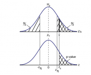
If the between-group variance is large enough that there is little or no overlap between groups, then your statistical test will reflect that by showing a low p -value . This means it is unlikely that the differences between these groups came about by chance.

Alternatively, if there is high within-group variance and low between-group variance, then your statistical test will reflect that with a high p -value. This means it is likely that any difference you measure between groups is due to chance.

Your choice of statistical test will be based on the type of variables and the level of measurement of your collected data .

• an estimate of the difference in average height between the two groups.
• a p -value showing how likely you are to see this difference if the null hypothesis of no difference is true.

Based on the outcome of your statistical test, you will have to decide whether to reject or fail to reject your null hypothesis.

In most cases you will use the p -value generated by your statistical test to guide your decision. And in most cases, your predetermined level of significance for rejecting the null hypothesis will be 0.05 – that is, when there is a less than 5% chance that you would see these results if the null hypothesis were true.

In some cases, researchers choose a more conservative level of significance, such as 0.01 (1%). This minimizes the risk of incorrectly rejecting the null hypothesis ( Type I error ).

The results of hypothesis testing will be presented in the results and discussion sections of your research paper , dissertation or thesis .

In the results section you should give a brief summary of the data and a summary of the results of your statistical test (for example, the estimated difference between group means and associated p -value). In the discussion , you can discuss whether your initial hypothesis was supported by your results or not.

In the formal language of hypothesis testing, we talk about rejecting or failing to reject the null hypothesis. You will probably be asked to do this in your statistics assignments.

However, when presenting research results in academic papers we rarely talk this way. Instead, we go back to our alternate hypothesis (in this case, the hypothesis that men are on average taller than women) and state whether the result of our test did or did not support the alternate hypothesis.

If your null hypothesis was rejected, this result is interpreted as “supported the alternate hypothesis.”

These are superficial differences; you can see that they mean the same thing.

You might notice that we don’t say that we reject or fail to reject the alternate hypothesis . This is because hypothesis testing is not designed to prove or disprove anything. It is only designed to test whether a pattern we measure could have arisen spuriously, or by chance.

If we reject the null hypothesis based on our research (i.e., we find that it is unlikely that the pattern arose by chance), then we can say our test lends support to our hypothesis . But if the pattern does not pass our decision rule, meaning that it could have arisen by chance, then we say the test is inconsistent with our hypothesis .

If you want to know more about statistics , methodology , or research bias , make sure to check out some of our other articles with explanations and examples.

• Normal distribution
• Descriptive statistics
• Measures of central tendency
• Correlation coefficient

Methodology

• Cluster sampling
• Stratified sampling
• Types of interviews
• Cohort study
• Thematic analysis

Research bias

• Implicit bias
• Cognitive bias
• Survivorship bias
• Availability heuristic
• Nonresponse bias
• Regression to the mean

Hypothesis testing is a formal procedure for investigating our ideas about the world using statistics. It is used by scientists to test specific predictions, called hypotheses , by calculating how likely it is that a pattern or relationship between variables could have arisen by chance.

A hypothesis states your predictions about what your research will find. It is a tentative answer to your research question that has not yet been tested. For some research projects, you might have to write several hypotheses that address different aspects of your research question.

A hypothesis is not just a guess — it should be based on existing theories and knowledge. It also has to be testable, which means you can support or refute it through scientific research methods (such as experiments, observations and statistical analysis of data).

Null and alternative hypotheses are used in statistical hypothesis testing . The null hypothesis of a test always predicts no effect or no relationship between variables, while the alternative hypothesis states your research prediction of an effect or relationship.

Cite this Scribbr article

If you want to cite this source, you can copy and paste the citation or click the “Cite this Scribbr article” button to automatically add the citation to our free Citation Generator.

Bevans, R. (2023, June 22). Hypothesis Testing | A Step-by-Step Guide with Easy Examples. Scribbr. Retrieved April 8, 2024, from https://www.scribbr.com/statistics/hypothesis-testing/

Is this article helpful?

Rebecca Bevans

Other students also liked, choosing the right statistical test | types & examples, understanding p values | definition and examples, what is your plagiarism score.

• school Campus Bookshelves
• menu_book Bookshelves
• perm_media Learning Objects
• login Login
• how_to_reg Request Instructor Account
• hub Instructor Commons
• Download Page (PDF)
• Download Full Book (PDF)
• Periodic Table
• Physics Constants
• Scientific Calculator
• Reference & Cite
• Tools expand_more
• Readability

selected template will load here

This action is not available.

7.6: Steps of the Hypothesis Testing Process

• Last updated
• Save as PDF
• Page ID 22073

• Michelle Oja
• Taft College

The process of testing hypotheses follows a simple four-step procedure. This process will be what we use for the remained of the textbook and course, and though the hypothesis and statistics we use will change, this process will not.

Step 1: State the Hypotheses

Your hypotheses are the first thing you need to lay out. Otherwise, there is nothing to test! You have to state the null hypothesis (which is what we test) and the research hypothesis (which is what we expect). These should be stated mathematically as they were presented above AND in words, explaining in normal English what each one means in terms of the research question.

Step 2: Find the Critical Values

Next, we formally lay out the criteria we will use to test our hypotheses. There are two pieces of information that inform our critical values: \(α\), wh ich determines how much of the area under the curve composes our rejection region, and the directionality of the test, which determines where the region will be.

Step 3: Compute the Test Statistic

Once we have our hypotheses and the standards we use to test them, we can collect data and calculate our test statistic . This step is where the vast majority of differences in future chapters will arise: different tests used for different data are calculated in different ways, but the way we use and interpret them remains the same.

Step 4: Make the Decision

Finally, once we have our calculated test statistic, we can compare it to our critical value and decide whether we should reject or fail to reject the null hypothesis. When we do this, we must interpret the decision in relation to our research question, stating what we concluded, what we based our conclusion on, and the specific statistics we obtained.

We will talk more about what is included in the write-up that explains the interpretation of the decision in relation to the research question, but remember that your answer is never just a number in behavioral statistics. And in Null Hypothesis Significance Testing, your answer is probably at least several sentences explaining the groups, what was measured, the results. and how it all relates to the research hypothesis.

Want to create or adapt books like this? Learn more about how Pressbooks supports open publishing practices.

11 Hypothesis Testing with One Sample

Student learning outcomes.

By the end of this chapter, the student should be able to:

• Be able to identify and develop the null and alternative hypothesis
• Identify the consequences of Type I and Type II error.
• Be able to perform an one-tailed and two-tailed hypothesis test using the critical value method
• Be able to perform a hypothesis test using the p-value method
• Be able to write conclusions based on hypothesis tests.

Introduction

Now we are down to the bread and butter work of the statistician: developing and testing hypotheses. It is important to   put this material in a broader context so that the method by which a hypothesis is formed is understood completely. Using textbook examples often clouds the real source of statistical hypotheses.

Statistical testing is part of a much larger process known as the scientific method. This method was developed more than two centuries ago as the accepted way that new knowledge could be created. Until then, and unfortunately even today, among some, “knowledge” could be created simply by some authority saying something was so, ipso dicta . Superstition and conspiracy theories were (are?) accepted uncritically.

The scientific method, briefly, states that only by following a careful and specific process can some assertion be included in the accepted body of knowledge. This process begins with a set of assumptions upon which a theory, sometimes called a model, is built. This theory, if it has any validity, will lead to predictions; what we call hypotheses.

As an example, in Microeconomics the theory of consumer choice begins with certain assumption concerning human behavior. From these assumptions a theory of how consumers make choices using indifference curves and the budget line. This theory gave rise to a very important prediction, namely, that there was an inverse relationship between price and quantity demanded. This relationship was known as the demand curve. The negative slope of the demand curve is really just a prediction, or a hypothesis, that can be tested with statistical tools.

Unless hundreds and hundreds of statistical tests of this hypothesis had not confirmed this relationship, the so-called Law of Demand would have been discarded years ago. This is the role of statistics, to test the hypotheses of various theories to determine if they should be admitted into the accepted body of knowledge; how we understand our world. Once admitted, however, they may be later discarded if new theories come along that make better predictions.

Not long ago two scientists claimed that they could get more energy out of a process than was put in. This caused a tremendous stir for obvious reasons. They were on the cover of Time and were offered extravagant sums to bring their research work to private industry and any number of universities. It was not long until their work was subjected to the rigorous tests of the scientific method and found to be a failure. No other lab could replicate their findings. Consequently they have sunk into obscurity and their theory discarded. It may surface again when someone can pass the tests of the hypotheses required by the scientific method, but until then it is just a curiosity. Many pure frauds have been attempted over time, but most have been found out by applying the process of the scientific method.

This discussion is meant to show just where in this process statistics falls. Statistics and statisticians are not necessarily in the business of developing theories, but in the business of testing others’ theories. Hypotheses come from these theories based upon an explicit set of assumptions and sound logic. The hypothesis comes first, before any data are gathered. Data do not create hypotheses; they are used to test them. If we bear this in mind as we study this section the process of forming and testing hypotheses will make more sense.

One job of a statistician is to make statistical inferences about populations based on samples taken from the population. Confidence intervals are one way to estimate a population parameter. Another way to make a statistical inference is to make a decision about the value of a specific parameter. For instance, a car dealer advertises that its new small truck gets 35 miles per gallon, on average. A tutoring service claims that its method of tutoring helps 90% of its students get an A or a B. A company says that women managers in their company earn an average of $60,000 per year.

A statistician will make a decision about these claims. This process is called ” hypothesis testing .” A hypothesis test involves collecting data from a sample and evaluating the data. Then, the statistician makes a decision as to whether or not there is sufficient evidence, based upon analyses of the data, to reject the null hypothesis.

In this chapter, you will conduct hypothesis tests on single means and single proportions. You will also learn about the errors associated with these tests.

Null and Alternative Hypotheses

The actual test begins by considering two hypotheses . They are called the null hypothesis and the alternative hypothesis . These hypotheses contain opposing viewpoints.

Since the null and alternative hypotheses are contradictory, you must examine evidence to decide if you have enough evidence to reject the null hypothesis or not. The evidence is in the form of sample data.

Table 1 presents the various hypotheses in the relevant pairs. For example, if the null hypothesis is equal to some value, the alternative has to be not equal to that value.

NOTE                                                                             

We want to test whether the mean GPA of students in American colleges is different from 2.0 (out of 4.0). The null and alternative hypotheses are:

We want to test if college students take less than five years to graduate from college, on the average. The null and alternative hypotheses are:

Outcomes and the Type I and Type II Errors

The four possible outcomes in the table are:

Each of the errors occurs with a particular probability. The Greek letters α and β represent the probabilities.

By way of example, the American judicial system begins with the concept that a defendant is “presumed innocent”. This is the status quo and is the null hypothesis. The judge will tell the jury that they can not find the defendant guilty unless the evidence indicates guilt beyond a “reasonable doubt” which is usually defined in criminal cases as 95% certainty of guilt. If the jury cannot accept the null, innocent, then action will be taken, jail time. The burden of proof always lies with the alternative hypothesis. (In civil cases, the jury needs only to be more than 50% certain of wrongdoing to find culpability, called “a preponderance of the evidence”).

The example above was for a test of a mean, but the same logic applies to tests of hypotheses for all statistical parameters one may wish to test.

The following are examples of Type I and Type II errors.

Type I error : Frank thinks that his rock climbing equipment may not be safe when, in fact, it really is safe.

Type II error : Frank thinks that his rock climbing equipment may be safe when, in fact, it is not safe.

Notice that, in this case, the error with the greater consequence is the Type II error. (If Frank thinks his rock climbing equipment is safe, he will go ahead and use it.)

This is a situation described as “accepting a false null”.

Type I error : The emergency crew thinks that the victim is dead when, in fact, the victim is alive. Type II error : The emergency crew does not know if the victim is alive when, in fact, the victim is dead.

The error with the greater consequence is the Type I error. (If the emergency crew thinks the victim is dead, they will not treat him.)

Distribution Needed for Hypothesis Testing

Particular distributions are associated with hypothesis testing.We will perform hypotheses tests of a population mean using a normal distribution or a Student’s t -distribution. (Remember, use a Student’s t -distribution when the population standard deviation is unknown and the sample size is small, where small is considered to be less than 30 observations.) We perform tests of a population proportion using a normal distribution when we can assume that the distribution is normally distributed. We consider this to be true if the sample proportion, p ‘ , times the sample size is greater than 5 and 1- p ‘ times the sample size is also greater then 5. This is the same rule of thumb we used when developing the formula for the confidence interval for a population proportion.

Hypothesis Test for the Mean

Going back to the standardizing formula we can derive the test statistic for testing hypotheses concerning means.

This gives us the decision rule for testing a hypothesis for a two-tailed test:

P-Value Approach

Both decision rules will result in the same decision and it is a matter of preference which one is used.

One and Two-tailed Tests

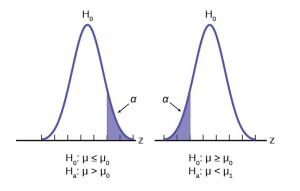
The claim would be in the alternative hypothesis. The burden of proof in hypothesis testing is carried in the alternative. This is because failing to reject the null, the status quo, must be accomplished with 90 or 95 percent significance that it cannot be maintained. Said another way, we want to have only a 5 or 10 percent probability of making a Type I error, rejecting a good null; overthrowing the status quo.

Figure 5 shows the two possible cases and the form of the null and alternative hypothesis that give rise to them.

Effects of Sample Size on Test Statistic

Table 3 summarizes test statistics for varying sample sizes and population standard deviation known and unknown.

A Systematic Approach for Testing A Hypothesis

A systematic approach to hypothesis testing follows the following steps and in this order. This template will work for all hypotheses that you will ever test.

• Set up the null and alternative hypothesis. This is typically the hardest part of the process. Here the question being asked is reviewed. What parameter is being tested, a mean, a proportion, differences in means, etc. Is this a one-tailed test or two-tailed test? Remember, if someone is making a claim it will always be a one-tailed test.
• Decide the level of significance required for this particular case and determine the critical value. These can be found in the appropriate statistical table. The levels of confidence typical for the social sciences are 90, 95 and 99. However, the level of significance is a policy decision and should be based upon the risk of making a Type I error, rejecting a good null. Consider the consequences of making a Type I error.
• Take a sample(s) and calculate the relevant parameters: sample mean, standard deviation, or proportion. Using the formula for the test statistic from above in step 2, now calculate the test statistic for this particular case using the parameters you have just calculated.
• Compare the calculated test statistic and the critical value. Marking these on the graph will give a good visual picture of the situation. There are now only two situations:

a.     The test statistic is in the tail: Cannot Accept the null, the probability that this sample mean (proportion) came from the hypothesized distribution is too small to believe that it is the real home of these sample data.

b.   The test statistic is not in the tail: Cannot Reject the null, the sample data are compatible with the hypothesized population parameter.

• Reach a conclusion. It is best to articulate the conclusion two different ways. First a formal statistical conclusion such as “With a 95 % level of significance we cannot accept the null hypotheses that the population mean is equal to XX (units of measurement)”. The second statement of the conclusion is less formal and states the action, or lack of action, required. If the formal conclusion was that above, then the informal one might be, “The machine is broken and we need to shut it down and call for repairs”.

All hypotheses tested will go through this same process. The only changes are the relevant formulas and those are determined by the hypothesis required to answer the original question.

Full Hypothesis Test Examples

Tests on means.

Jeffrey, as an eight-year old, established a mean time of 16.43 seconds for swimming the 25-yard freestyle, with a standard deviation of 0.8 seconds . His dad, Frank, thought that Jeffrey could swim the 25-yard freestyle faster using goggles. Frank bought Jeffrey a new pair of expensive goggles and timed Jeffrey for 15 25-yard freestyle swims . For the 15 swims, Jeffrey’s mean time was 16 seconds. Frank thought that the goggles helped Jeffrey to swim faster than the 16.43 seconds. Conduct a hypothesis test using a preset α = 0.05.

Solution – Example 6

Set up the Hypothesis Test:

Since the problem is about a mean, this is a test of a single population mean . Set the null and alternative hypothesis:

In this case there is an implied challenge or claim. This is that the goggles will reduce the swimming time. The effect of this is to set the hypothesis as a one-tailed test. The claim will always be in the alternative hypothesis because the burden of proof always lies with the alternative. Remember that the status quo must be defeated with a high degree of confidence, in this case 95 % confidence. The null and alternative hypotheses are thus:

For Jeffrey to swim faster, his time will be less than 16.43 seconds. The “<” tells you this is left-tailed. Determine the distribution needed:

Distribution for the test statistic:

The sample size is less than 30 and we do not know the population standard deviation so this is a t-test and the proper formula is:

Our step 2, setting the level of significance, has already been determined by the problem, .05 for a 95 % significance level. It is worth thinking about the meaning of this choice. The Type I error is to conclude that Jeffrey swims the 25-yard freestyle, on average, in less than 16.43 seconds when, in fact, he actually swims the 25-yard freestyle, on average, in 16.43 seconds. (Reject the null hypothesis when the null hypothesis is true.) For this case the only concern with a Type I error would seem to be that Jeffery’s dad may fail to bet on his son’s victory because he does not have appropriate confidence in the effect of the goggles.

To find the critical value we need to select the appropriate test statistic. We have concluded that this is a t-test on the basis of the sample size and that we are interested in a population mean. We can now draw the graph of the t-distribution and mark the critical value (Figure 6). For this problem the degrees of freedom are n-1, or 14. Looking up 14 degrees of freedom at the 0.05 column of the t-table we find 1.761. This is the critical value and we can put this on our graph.

Step 3 is the calculation of the test statistic using the formula we have selected.

We find that the calculated test statistic is 2.08, meaning that the sample mean is 2.08 standard deviations away from the hypothesized mean of 16.43.

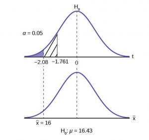
Step 4 has us compare the test statistic and the critical value and mark these on the graph. We see that the test statistic is in the tail and thus we move to step 4 and reach a conclusion. The probability that an average time of 16 minutes could come from a distribution with a population mean of 16.43 minutes is too unlikely for us to accept the null hypothesis. We cannot accept the null.

Step 5 has us state our conclusions first formally and then less formally. A formal conclusion would be stated as: “With a 95% level of significance we cannot accept the null hypothesis that the swimming time with goggles comes from a distribution with a population mean time of 16.43 minutes.” Less formally, “With 95% significance we believe that the goggles improves swimming speed”

If we wished to use the p-value system of reaching a conclusion we would calculate the statistic and take the additional step to find the probability of being 2.08 standard deviations from the mean on a t-distribution. This value is .0187. Comparing this to the α-level of .05 we see that we cannot accept the null. The p-value has been put on the graph as the shaded area beyond -2.08 and it shows that it is smaller than the hatched area which is the alpha level of 0.05. Both methods reach the same conclusion that we cannot accept the null hypothesis.

Jane has just begun her new job as on the sales force of a very competitive company. In a sample of 16 sales calls it was found that she closed the contract for an average value of $108 with a standard deviation of 12 dollars. Test at 5% significance that the population mean is at least $100 against the alternative that it is less than 100 dollars. Company policy requires that new members of the sales force must exceed an average of $100 per contract during the trial employment period. Can we conclude that Jane has met this requirement at the significance level of 95%?

Solution – Example 7

STEP 1 : Set the Null and Alternative Hypothesis.

STEP 2 : Decide the level of significance and draw the graph (Figure 7) showing the critical value.

STEP 3 : Calculate sample parameters and the test statistic.

STEP 4 : Compare test statistic and the critical values

STEP 5 : Reach a Conclusion

The test statistic is a Student’s t because the sample size is below 30; therefore, we cannot use the normal distribution. Comparing the calculated value of the test statistic and the critical value of t ( t a ) at a 5% significance level, we see that the calculated value is in the tail of the distribution. Thus, we conclude that 108 dollars per contract is significantly larger than the hypothesized value of 100 and thus we cannot accept the null hypothesis. There is evidence that supports Jane’s performance meets company standards.

Again we will follow the steps in our analysis of this problem.

Solution – Example 8

STEP 1 : Set the Null and Alternative Hypothesis. The random variable is the quantity of fluid placed in the bottles. This is a continuous random variable and the parameter we are interested in is the mean. Our hypothesis therefore is about the mean. In this case we are concerned that the machine is not filling properly. From what we are told it does not matter if the machine is over-filling or under-filling, both seem to be an equally bad error. This tells us that this is a two-tailed test: if the machine is malfunctioning it will be shutdown regardless if it is from over-filling or under-filling. The null and alternative hypotheses are thus:

STEP 2 : Decide the level of significance and draw the graph showing the critical value.

This problem has already set the level of significance at 99%. The decision seems an appropriate one and shows the thought process when setting the significance level. Management wants to be very certain, as certain as probability will allow, that they are not shutting down a machine that is not in need of repair. To draw the distribution and the critical value, we need to know which distribution to use. Because this is a continuous random variable and we are interested in the mean, and the sample size is greater than 30, the appropriate distribution is the normal distribution and the relevant critical value is 2.575 from the normal table or the t-table at 0.005 column and infinite degrees of freedom. We draw the graph and mark these points (Figure 8).

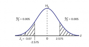
STEP 3 : Calculate sample parameters and the test statistic. The sample parameters are provided, the sample mean is 7.91 and the sample variance is .03 and the sample size is 35. We need to note that the sample variance was provided not the sample standard deviation, which is what we need for the formula. Remembering that the standard deviation is simply the square root of the variance, we therefore know the sample standard deviation, s, is 0.173. With this information we calculate the test statistic as -3.07, and mark it on the graph.

STEP 4 : Compare test statistic and the critical values Now we compare the test statistic and the critical value by placing the test statistic on the graph. We see that the test statistic is in the tail, decidedly greater than the critical value of 2.575. We note that even the very small difference between the hypothesized value and the sample value is still a large number of standard deviations. The sample mean is only 0.08 ounces different from the required level of 8 ounces, but it is 3 plus standard deviations away and thus we cannot accept the null hypothesis.

Three standard deviations of a test statistic will guarantee that the test will fail. The probability that anything is within three standard deviations is almost zero. Actually it is 0.0026 on the normal distribution, which is certainly almost zero in a practical sense. Our formal conclusion would be “ At a 99% level of significance we cannot accept the hypothesis that the sample mean came from a distribution with a mean of 8 ounces” Or less formally, and getting to the point, “At a 99% level of significance we conclude that the machine is under filling the bottles and is in need of repair”.

Media Attributions

• Type1Type2Error
• HypTestFig2
• HypTestFig3
• HypTestPValue
• OneTailTestFig5
• HypTestExam7
• HypTestExam8

Quantitative Analysis for Business Copyright © by Margo Bergman is licensed under a Creative Commons Attribution-NonCommercial-ShareAlike 4.0 International License , except where otherwise noted.

Share This Book

User Preferences

Content preview.

Arcu felis bibendum ut tristique et egestas quis:

• Ut enim ad minim veniam, quis nostrud exercitation ullamco laboris
• Duis aute irure dolor in reprehenderit in voluptate
• Excepteur sint occaecat cupidatat non proident

Keyboard Shortcuts

7.4.1 - hypothesis testing, five step hypothesis testing procedure section  .

In the remaining lessons, we will use the following five step hypothesis testing procedure. This is slightly different from the five step procedure that we used when conducting randomization tests. 

• Check assumptions and write hypotheses.  The assumptions will vary depending on the test. In this lesson we'll be confirming that the sampling distribution is approximately normal by visually examining the randomization distribution. In later lessons you'll learn more objective assumptions. The null and alternative hypotheses will always be written in terms of population parameters; the null hypothesis will always contain the equality (i.e., \(=\)).
• Calculate the test statistic.  Here, we'll be using the formula below for the general form of the test statistic.
• Determine the p-value.  The p-value is the area under the standard normal distribution that is more extreme than the test statistic in the direction of the alternative hypothesis.
• Make a decision.  If \(p \leq \alpha\) reject the null hypothesis. If \(p>\alpha\) fail to reject the null hypothesis.
• State a "real world" conclusion.  Based on your decision in step 4, write a conclusion in terms of the original research question.

General Form of a Test Statistic Section  

When using a standard normal distribution (i.e., z distribution), the test statistic is the standardized value that is the boundary of the p-value. Recall the formula for a z score: \(z=\frac{x-\overline x}{s}\). The formula for a test statistic will be similar. When conducting a hypothesis test the sampling distribution will be centered on the null parameter and the standard deviation is known as the standard error.

This formula puts our observed sample statistic on a standard scale (e.g., z distribution). A z score tells us where a score lies on a normal distribution in standard deviation units. The test statistic tells us where our sample statistic falls on the sampling distribution in standard error units.

7-Hypothesis Test

What is hypothesis testing.

• It is practically impossible to observe every individual in a population. Therefore, samples are collected to analyse population behaviour.
• Hypothesis testing is a statistical procedure that helps us to draw inferences about the population by using sample data.

• A hypothesis test is a method of making decisions or inferences from sample data (evidence)
• A hypothesis test is a statistical method that uses sample data to evaluate a hypothesis about a population.
• Hypothesis testing is one of the most commonly used inferential procedures. Details of a hypothesis test change from one situation to another, but the general process remains constant.
• Concepts of z-scores, probability & sample mean are used to create a new statistical procedure known as a hypothesis test.

Steps of a Hypothesis Test

1. collect data and compute sample statistics..

• The raw data from the sample are summarized with the appropriate statistics
• Compute the sample mean. Now it is possible to compare the sample mean (the data) with the null hypothesis.

Now we calculate a z-score that identifies where our sample mean is located in this hypothesized distribution. The z-score formula for a sample mean

• In place of the Z score, other statistical scores (t score etc.) can also be calculated depending on the nature of the distribution of data.

2. State the hypothesis

• State a hypothesis about the unknown population.
• We state two opposing hypotheses.

(a) The null hypothesis (H 0 )

• The null hypothesis states that there is no change, no effect, no difference, and nothing happened, hence the name null.
• The null hypothesis states that the treatment has no effect.
• It assumes that in the general population, there is no change, no difference, or no relationship.
• In the context of an experiment, H 0 predicts that the independent variable (treatment) has no effect on the dependent variable (scores) for the population.
• The null hypothesis is identified by the symbol H 0 . (The H stands for hypothesis, and the zero subscripts indicate that this is the zero-effect hypothesis.)

Hypothesis H 0 :

• The sample mean = Population mean
• μ sample                      =        μ population

(b) The alternative hypothesis (H 1 )

• The second hypothesis is simply the opposite of the null hypothesis, and it is called the scientific, or alternative, hypothesis (H1 ).
• It states that there is a change, a difference, or a relationship for the general population.
• This hypothesis states that the treatment has an effect on the dependent variable

Hypothesis H 1 :

• μ sample ≠ μ population
• In the context of an experiment, H1 predicts that the independent variable (treatment) does have an effect on the dependent variable.

Examples: Null & Alternate Hypothesis test

• Doctors want to find out if the new medicine will have any side effects. The parameters considered for understudy were the pulse rate of the patients who have taken the medicine.

What are the hypotheses to test whether the pulse rate will be different from the mean pulse rate of 82 beats per minute?

• Null Hypothesis: H 0 μ = 82
• Alternate Hypothesis: H 1 μ ≠ 82
• The engineer wants to reduce the electricity bill by using a spray type of desert cooler in summer in houses. If the average monthly Electric bill is Rs 1500 per month.

What are the hypotheses to test whether the electric bill will be different from the average electric bill of Rs 1500 per month?

• Null Hypothesis: H 0          μ =1500
• Alternate Hypothesis: H 1 μ ≠ 1500
• The engineer invents an electric circuit to increase the average (Petrol consumed in Liter per KM travel) of a motorcycle. If the average before fitting the device was 55 KM/litre,

What are the hypotheses to test whether the Motorcycle average will be different from the average of 55 KM/litre?

• Null Hypothesis: H 0 μ =55
• Alternate Hypothesis: H 1 μ ≠ 55

3. Set the criteria for a decision

• Data from the sample is used to evaluate the reliability of the null hypothesis.
• The data will either provide support for the null hypothesis or tend to disprove the null hypothesis.
• First selected a specific probability value, which is known as the level of significance, or the alpha level, for the hypothesis test.
• α = .05 (5%)
• α = .01 (1%)
• α = .001 (0.1%).
• For example, with α = .05, we separate the most unlikely 5% of the sample means (the extreme values) from the most likely 95% of the sample means (the central values)
• The alpha (α) value is a small probability that is used to identify the low-probability samples.
• With the help of the alpha-level decision, boundaries are calculated.

The Alpha Level

• The alpha level, or the level of significance, is a probability value that is used to define the concept of “very unlikely” in a hypothesis test.
• The critical region is composed of the extreme sample values that are very unlikely (as defined by the alpha level) to be obtained if the null hypothesis is true.
• See the below figure, α = Area A + Area B. This area is represented in grey colour. It is called a critical region. Corresponding critical values are calculated from the α level.

• The boundaries for the critical region are determined by the alpha level. If sample data fall in the critical region, the null hypothesis is rejected
• If Z calculated value is within the critical zone – Hypothesis H 0 will be rejected
• Zcalculated = -2.65, it is below the Zcritical = – 1.96
• It falls inside the critical region.
• Hence H 0 is rejected.

• Zcalculated = + 2.01 , it is above the Zcritical = + 1.96
• It falls inside the critical region
• Hence H 0 is rejected

If Z calculated value is outside the critical zone – Hypothesis H 0 will be accepted

• Zcalculated = -1.21, it is above the Zcritical = – 1.96
• It falls outside the critical region
• Hence H 0 is accepted

4. Determine critical region boundaries of separation

For α = .05, determine critical region boundaries

• With α = .05, for example, the boundaries separate the extreme 5% from the middle 95%. Because the extreme 5% is split between two tails of the distribution, there is exactly 2.5% (or 0.0250) in each tail.
• Explanation of α = .05 in terms of Probability distribution :-

• Explanation of α = .05 in terms of Area under Probability distribution curve :-

• Explanation of α = .05 on Normal distribution curve (Probability distribution curve):-

In the normal Z table , look up a proportion of 0.0250 in the column and find the z-score value.

• For α = .0250 , z = 1.96
• For any normal distribution, the tails of the distribution are beyond z = +1.96 and z = –1.96. values define the boundaries of the critical region for a hypothesis test using α = .05

For α = .01, determine critical region boundaries

• An alpha level of α = .01 means that 1% or .0100 is split between the two tails.
• Explanation of α = .01 in terms of Probability distribution :-

• Explanation of α = .01 in terms of the Area of the Probability distribution curve :-

• Explanation of α = .01 on Normal distribution curve (Probability distribution curve):-

• In the normal Z table , look up a proportion of 0.005 in the column and find the z-score value.
• For α = .005 , z = 3.30
• For any normal distribution, tails of the distribution beyond z = +3.30 and z = –3.30, values define the boundaries of the critical region for a hypothesis test using α = .01

5. Take a decision about the Hypothesis

Condition 1: The sample data outside the critical region .

• If the Z calculated value is in the Critical Zone, the sample is not consistent with H 0 and the decision will be to reject the null hypothesis.
• The sample mean is reasonably away from the population mean
• Treatment did have an effect on the sample wrt population
• There is a change in the sample in comparison to the population
• There is a difference in a sample from the population etc.

Condition 2: The sample data are located within the critical region.

• If Z calculated  value is NOT in the Critical zone, sample data do not provide strong evidence that the null hypothesis is wrong, our conclusion is to accept the null hypothesis H 0
• In this case, the sample mean is reasonably close to the population mean
• Treatment did NOT have an effect on the sample wrt population
• There is NO change in the sample in comparison to the population
• There is NO difference in a sample from the population etc.

Refer: ENGINEERING STATISTICS HANDBOOK (NIST)

• https://matistics.com/statistics-data-variables/
• https://matistics.com/descriptive-statistics/
• https://matistics.com/1-1-measurement-scale/
• https://matistics.com/point-biserial-correlation-and-biserial-correlation/
• https://matistics.com/2-0-statistics-distributions/
• https://matistics.com/1-2-statistics-population-and-sample/
• https://matistics.com/7-hypothesis-testing/
• https://matistics.com/8-errors-in-hypothesis-testing/
• https://matistics.com/9-one-tailed-hypothesis-test/
• https://matistics.com/10-statistical-power/
• https://matistics.com/11-t-statistics/
• https://matistics.com/12-hypothesis-t-test-one-sample/
• https://matistics.com/13-hypothesis-t-test-2-sample/
• https://matistics.com/14-t-test-for-two-related-samples/
• https://matistics.com/15-analysis-of-variance-anova-independent-measures/
• https://matistics.com/16-anova-repeated-measures/
• https://matistics.com/17-two-factor-anova-independent-measures/
• https://matistics.com/18-correlation/
• https://matistics.com/19-regression/
• https://matistics.com/20-chi-square-statistic/
• https://matistics.com/21-binomial-test/

Related Posts

17 – two-factor anova -independent measures.

20- Chi-Square Statistic

1.2 – Statistics: Population and Sample

9-One tailed Hypothesis test

15-Analysis of Variance (ANOVA) Independent-Measures

Hypothesis t-test: Two Independent Samples

2.0 – Statistical distributions

19 – Regression

Leave a Comment Cancel Reply

Your email address will not be published. Required fields are marked *

Save my name, email, and website in this browser for the next time I comment.

Insert/edit link

Enter the destination URL

Or link to existing content

• Privacy Overview
• Strictly Necessary Cookies
• Privacy Policy

This website uses cookies so that we can provide you with the best user experience possible. Cookie information is stored in your browser and performs functions such as recognising you when you return to our website and helping our team to understand which sections of the website you find most interesting and useful.

Strictly Necessary Cookie should be enabled at all times so that we can save your preferences for cookie settings.

If you disable this cookie, we will not be able to save your preferences. This means that every time you visit this website you will need to enable or disable cookies again.

More information about our Privacy Policy

JMP Learning Library

Hypothesis test and confidence interval for proportions, estimate and perform a hypothesis test for a population proportion., step-by-step guide, where in jmp.

• Analyze > Distribution

Video tutorial

Want them all.

Download all the One-Page PDF Guides combined into one bundle.