presentation analysis and interpretation of data about covid 19

The COVID-19 pandemic in data visualizations

A man runs past white flags representing Americans who have died of COVID-19 on 20 acres of the National Mall in Washington, U.S., September 17, 2021. Image:  REUTERS/Joshua Roberts - RC2ORP90E3YF

.chakra .wef-1c7l3mo{-webkit-transition:all 0.15s ease-out;transition:all 0.15s ease-out;cursor:pointer;-webkit-text-decoration:none;text-decoration:none;outline:none;color:inherit;}.chakra .wef-1c7l3mo:hover,.chakra .wef-1c7l3mo[data-hover]{-webkit-text-decoration:underline;text-decoration:underline;}.chakra .wef-1c7l3mo:focus,.chakra .wef-1c7l3mo[data-focus]{box-shadow:0 0 0 3px rgba(168,203,251,0.5);} Andrew Berkley

John letzing.

.chakra .wef-9dduvl{margin-top:16px;margin-bottom:16px;line-height:1.388;font-size:1.25rem;}@media screen and (min-width:56.5rem){.chakra .wef-9dduvl{font-size:1.125rem;}} Explore and monitor how .chakra .wef-15eoq1r{margin-top:16px;margin-bottom:16px;line-height:1.388;font-size:1.25rem;color:#F7DB5E;}@media screen and (min-width:56.5rem){.chakra .wef-15eoq1r{font-size:1.125rem;}} COVID-19 is affecting economies, industries and global issues

.chakra .wef-1nk5u5d{margin-top:16px;margin-bottom:16px;line-height:1.388;color:#2846F8;font-size:1.25rem;}@media screen and (min-width:56.5rem){.chakra .wef-1nk5u5d{font-size:1.125rem;}} Get involved with our crowdsourced digital platform to deliver impact at scale

Stay up to date:.

Listen to the article

• It’s been roughly a year-and-a-half since COVID-19 was declared a pandemic.
• The World Economic Forum has been tracing its impact with data visualizations.
• These excerpts reflect mounting caseloads and vaccination progress.

It’s been slightly more than a year-and-a-half since the WHO declared COVID-19 a global pandemic. For many people, it may be hard to believe it hasn’t been longer.

The global health crisis has changed the ways we work , travel , learn and socialize . It’s exacted an official death toll nearly equal to the population of Ireland (though that’s probably an undercount ), permanently altered countless other lives , and exposed flaws in health care systems and the social fabric .

But it's also prompted a period of scientific triumph, as vaccines have been developed at a relatively breathtaking pace ( though not everyone with the ability to take one has).

The World Economic Forum has created a number of data visualizations tracing the pandemic's impact . The following are selected excerpts.

The spread of Covid-19

The first cases of what would later be identified as the coronavirus that causes COVID-19 were reported in China in late 2019. It quickly spread to multiple countries, and by the middle of this month there were about 226 million reported cases globally. Each country’s official caseload over time is represented here by expanding red dots:

Shifting hot spots

The spread of COVID-19 has been uneven within the US. New York City was an early epicenter last year, though other areas including Florida have more recently become hot spots. Official caseload levels over time are again represented here by expanding dots, but this time designated according to county:

The global response

Governments around the world implemented travel restrictions , closed schools , and started contact tracing efforts as the virus spread. In many instances these measures waxed and waned in terms of severity depending on the situation. Here, the darker red a country becomes, the more severe the measures over time – and the lighter they get, the less severe:

And then, Covid-19 vaccines

In some places, vaccination efforts have stalled in recent months amid complacency and skepticism. In others, particularly in Africa , vaccines simply haven’t been made widely available yet. Here, countries turn from white to progressively darker green as the percentage of the population fully vaccinated increases over time:

The Delta variant seems to have made herd immunity unlikely in most countries, at least for now. While predicted future scenarios vary, most experts appear to agree on at least two things: COVID-19 is here to stay, and our ability to contain it will depend on the choices we make.

For more context, here are links to further reading from the World Economic Forum's Strategic Intelligence platform :

• A third shot is now being offered in several countries where people have already been fortunate enough to be fully vaccinated. This analysis delves into whether or not that’s even necessary. ( The Conversation )
• Latin America has been hit especially hard by the pandemic, according to this piece, making it even more difficult for the region to pursue rapid decarbonization and build climate resilience. ( Project Syndicate )
• The core logic of China’s COVID-19 containment policy has been “zero tolerance,” according to this piece. That’s required massive efforts from nearly every part of society, to do things like complete coronavirus testing for all 11 million residents of Wuhan within 72 hours. ( The Diplomat )
• Sixteen reasons why you should get vaccinated. Among those listed in this piece: by being fully vaccinated your risk of COVID-19 infection is reduced by five times, and your risk of requiring hospitalization if infected is reduced by 10 times. ( Harvard Kennedy School )
• Winter worries. As the change in seasons approaches and people head indoors, experts are concerned more contagious variants of the coronavirus could emerge, according to this piece. The upshot: rules and restrictions will be around indefinitely. ( Der Spiegel )

On the Strategic Intelligence platform, you can find feeds of expert analysis related to COVID-19 , Vaccination , and hundreds of additional topics. You’ll need to register to view.

Don't miss any update on this topic

Create a free account and access your personalized content collection with our latest publications and analyses.

License and Republishing

World Economic Forum articles may be republished in accordance with the Creative Commons Attribution-NonCommercial-NoDerivatives 4.0 International Public License, and in accordance with our Terms of Use.

The views expressed in this article are those of the author alone and not the World Economic Forum.

The Agenda .chakra .wef-n7bacu{margin-top:16px;margin-bottom:16px;line-height:1.388;font-weight:400;} Weekly

A weekly update of the most important issues driving the global agenda

.chakra .wef-1dtnjt5{display:-webkit-box;display:-webkit-flex;display:-ms-flexbox;display:flex;-webkit-align-items:center;-webkit-box-align:center;-ms-flex-align:center;align-items:center;-webkit-flex-wrap:wrap;-ms-flex-wrap:wrap;flex-wrap:wrap;} More on Health and Healthcare Systems .chakra .wef-nr1rr4{display:-webkit-inline-box;display:-webkit-inline-flex;display:-ms-inline-flexbox;display:inline-flex;white-space:normal;vertical-align:middle;text-transform:uppercase;font-size:0.75rem;border-radius:0.25rem;font-weight:700;-webkit-align-items:center;-webkit-box-align:center;-ms-flex-align:center;align-items:center;line-height:1.2;-webkit-letter-spacing:1.25px;-moz-letter-spacing:1.25px;-ms-letter-spacing:1.25px;letter-spacing:1.25px;background:none;padding:0px;color:#B3B3B3;-webkit-box-decoration-break:clone;box-decoration-break:clone;-webkit-box-decoration-break:clone;}@media screen and (min-width:37.5rem){.chakra .wef-nr1rr4{font-size:0.875rem;}}@media screen and (min-width:56.5rem){.chakra .wef-nr1rr4{font-size:1rem;}} See all

Market failures cause antibiotic resistance. Here's how to address them

Katherine Klemperer and Anthony McDonnell

April 25, 2024

Equitable healthcare is the industry's north star. Here's how AI can get us there

Vincenzo Ventricelli

Bird flu spread a ‘great concern’, plus other top health stories

Shyam Bishen

April 24, 2024

This Earth Day we consider the impact of climate change on human health

Shyam Bishen and Annika Green

April 22, 2024

Scientists have invented a method to break down 'forever chemicals' in our drinking water. Here’s how

Johnny Wood

April 17, 2024

Young people are becoming unhappier, a new report finds

• Open access
• Published: 18 April 2024

The predictive power of data: machine learning analysis for Covid-19 mortality based on personal, clinical, preclinical, and laboratory variables in a case–control study

• Maryam Seyedtabib   ORCID: orcid.org/0000-0003-1599-9374 1 ,
• Roya Najafi-Vosough   ORCID: orcid.org/0000-0003-2871-5748 2 &
• Naser Kamyari   ORCID: orcid.org/0000-0001-6245-5447 3  

BMC Infectious Diseases volume  24 , Article number:  411 ( 2024 ) Cite this article

249 Accesses

1 Altmetric

Metrics details

Background and purpose

The COVID-19 pandemic has presented unprecedented public health challenges worldwide. Understanding the factors contributing to COVID-19 mortality is critical for effective management and intervention strategies. This study aims to unlock the predictive power of data collected from personal, clinical, preclinical, and laboratory variables through machine learning (ML) analyses.

A retrospective study was conducted in 2022 in a large hospital in Abadan, Iran. Data were collected and categorized into demographic, clinical, comorbid, treatment, initial vital signs, symptoms, and laboratory test groups. The collected data were subjected to ML analysis to identify predictive factors associated with COVID-19 mortality. Five algorithms were used to analyze the data set and derive the latent predictive power of the variables by the shapely additive explanation values.

Results highlight key factors associated with COVID-19 mortality, including age, comorbidities (hypertension, diabetes), specific treatments (antibiotics, remdesivir, favipiravir, vitamin zinc), and clinical indicators (heart rate, respiratory rate, temperature). Notably, specific symptoms (productive cough, dyspnea, delirium) and laboratory values (D-dimer, ESR) also play a critical role in predicting outcomes. This study highlights the importance of feature selection and the impact of data quantity and quality on model performance.

This study highlights the potential of ML analysis to improve the accuracy of COVID-19 mortality prediction and emphasizes the need for a comprehensive approach that considers multiple feature categories. It highlights the critical role of data quality and quantity in improving model performance and contributes to our understanding of the multifaceted factors that influence COVID-19 outcomes.

Peer Review reports

Introduction

The World Health Organization (WHO) has declared COVID-19 a global pandemic in March 2020 [ 1 ]. The first cases of SARSCoV-2, a new severe acute respiratory syndrome coronavirus, were detected in Wuhan, China, and rapidly spread to become a global public health problem [ 2 ]. The clinical presentation and symptoms of COVID-19 may be similar to those of Middle East Respiratory Syndrome (MERS) and Severe Acute Respiratory Syndrome (SARS), however the rate of spread is higher [ 3 ]. By December 31, 2022, the pandemic had caused more than 729 million cases and nearly 6.7 million deaths (0.92%) were confirmed in 219 countries worldwide [ 4 ]. For many countries, figuring out what measures to take to prevent death or serious illness is a major challenge. Due to the complexity of transmission and the lack of proven treatments, COVID-19 is a major challenge worldwide [ 5 , 6 ]. In middle- and low-income countries, the situation is even more catastrophic due to high illiteracy rates, a very poor health care system, and lack of intensive care units [ 5 ]. In addition, understanding the factors contributing to COVID-19 mortality is critical for effective management and intervention strategies [ 6 ].

Numerous studies have shown several factors associated with COVID-19 outcomes, including socioeconomic, environmental, individual demographic, and health factors [ 7 , 8 , 9 ]. Risk factors for COVID -19 mortality vary by study and population studied [ 10 ]. Age [ 11 , 12 ], comorbidities such as hypertension, cardiovascular disease, diabetes, and COPD [ 13 , 14 , 15 ], sex [ 13 ], race/ethnicity [ 11 ], dementia, and neurologic disease [ 16 , 17 ], are some of the factors associated with COVID-19 mortality. Laboratory factors such as elevated levels of inflammatory markers, lymphopenia, elevated creatinine levels, and ALT are also associated with COVID-19 mortality [ 5 , 18 ]. Understanding these multiple risk factors is critical to accurately diagnose and treat COVID-19 patients.

Accurate diagnosis and treatment of the disease requires a comprehensive assessment that considers a variety of factors. These factors include personal factors such as medical history, lifestyle, and genetics; clinical factors such as observations on physical examinations and physician reports; preclinical factors such as early detection through screening or surveillance; laboratory factors such as results of diagnostic tests and medical imaging; and patient-reported signs and symptoms. However, the variety of characteristics associated with COVID-19 makes it difficult for physicians to accurately classify COVID-19 patients during the pandemic.

In today's digital transformation era, machine learning plays a vital role in various industries, including healthcare, where substantial data is generated daily [ 19 , 20 , 21 ]. Numerous studies have explored machine learning (ML) and explainable artificial intelligence (AI) in predicting COVID-19 prognosis and diagnosis [ 22 , 23 , 24 , 25 ]. Chadaga et al. have developed decision support systems and triage prediction systems using clinical markers and biomarkers [ 22 , 23 ]. Similarly, Khanna et al. have developed a ML and explainable AI system for COVID-19 triage prediction [ 24 ]. Zoabi has also made contributions in this field, developing ML models that predict COVID-19 test results with high accuracy based on a small number of features such as gender, age, contact with an infected person and initial clinical symptoms [ 25 ]. These studies emphasize the potential of ML and explainable AI to improve COVID-19 prediction and diagnosis. Nonetheless, the efficacy of ML algorithms heavily relies on the quality and quantity of data utilized for training. Recent research has indicated that deep learning algorithms' performance can be significantly enhanced compared to traditional ML methods by increasing the volume of data used [ 26 ]. However, it is crucial to acknowledge that the impact of data volume on model performance can vary based on data characteristics and experimental setup, highlighting the need for careful consideration and analysis when selecting data for model training. While the studies emphasize the importance of features in training ML algorithms for COVID-19 prediction and diagnosis, additional research is required on methods to enhance the interpretability of features.

Therefore, the primary aim of this study is to identify the key factors associated with mortality in COVID -19 patients admitted to hospitals in Abadan, Iran. For this purpose, seven categories of factors were selected, including demographic, clinical and conditions, comorbidities, treatments, initial vital signs, symptoms, and laboratory tests, and machine learning algorithms were employed. The predictive power of the data was assessed using 139 predictor variables across seven feature sets. Our next goal is to improve the interpretability of the extracted important features. To achieve this goal, we will utilize the innovative SHAP analysis, which illustrates the impact of features through a diagram.

Materials and methods

Study population and data collection.

Using data from the COVID-19 hospital-based registry database, a retrospective study was conducted from April 2020 to December 2022 at Ayatollah Talleghani Hospital (a COVID‑19 referral center) in Abadan City, Iran.

A total of 14,938 patients were initially screened for eligibility for the study. Of these, 9509 patients were excluded because their transcriptase polymerase chain reaction (RT-PCR) test results were negative or unspecified. The exclusion of patients due to incomplete or missing data is a common issue in medical research, particularly in the use of electronic medical records (EMRs) [ 27 ]. In addition, 1623 patients were excluded because their medical records contained more than 70% incomplete or missing data. In addition, patients younger than 18 years were not included in the study. The criterion for excluding 1623 patients due to "70% incomplete or missing data" means that the medical records of these patients did not contain at least 30% of the data required for a meaningful analysis. This threshold was set to ensure that the dataset used for the study contained a sufficient amount of complete and reliable information to draw accurate conclusions. Incomplete or missing data in a medical record may relate to key variables such as patient demographics, symptoms, lab results, treatment information, outcomes, or other data points important to the research. Insufficient data can affect the validity and reliability of study results and lead to potential bias or inaccuracies in the findings. It is important to exclude such incomplete records to maintain the quality and integrity of the research findings and to ensure that the conclusions drawn are based on robust and reliable data. After these exclusions, 3806 patients remained. Of these patients, 474 died due to COVID -19, while the remaining 3332 patients recovered and were included in the control group. To obtain a balanced sample, the control group was selected with a propensity score matching (PSM). The PSM refers to a statistical technique used to create a balanced comparison group by matching individuals in the control group (in this case, the survived group) with individuals in the case group (in this case, the deceased group) based on their propensity scores. In this study, the propensity scores for each person represented the probability of death (coded as a binary outcome; survived = 0, deceased = 1) calculated from a set of covariates (demographic factors) using the matchit function from the MatchIt library. Two individuals, one from the deceased group and one from the survived group, are considered matched if the difference between their propensity scores is small. Non-matching participants are discarded. The matching aims to reduce bias by making the distribution of observed characteristics similar between groups, which ultimately improves the comparability of groups in observational studies [ 28 ]. In total, the study included 1063 COVID-19 patients who belonged to either the deceased group (case = 474) or the survived group (control = 589) (Fig.  1 ).

Flowchart describing the process of patient selection

In the COVID‑19 hospital‑based registry database, one hundred forty primary features in eight main classes including patient’s demographics (eight features), clinical and conditions features (16 features), comorbidities (18 features), treatment (17 features), initial vital sign (14 features), symptoms during hospitalization (31 features), laboratory results (35 features), and an output (0 for survived and 1 for deceased) was recorded for COVID-19 patients. The main features included in the hospital-based COVID-19 registry database are provided in Appendix Table  1 .

To ensure the accuracy of the recorded information, discharged patients or their relatives were called and asked to review some of the recorded information (demographic information, symptoms, and medical history). Clinical symptoms and vital signs were referenced to the first day of hospitalization (at admission). Laboratory test results were also referenced to the patient’s first blood sample at the time of hospitalization.

The study analyzed 140 variables in patients' records, normalizing continuous variables and creating a binary feature to categorize patients based on outcomes. To address the issue of an imbalanced dataset, the Synthetic Minority Over-sampling Technique (SMOTE) was utilized. Some classes were combined to simplify variables. For missing data, an imputation technique was applied, assuming a random distribution [ 29 ]. Little's MCAR test was performed with the naniar package to assess whether missing data in a dataset is missing completely at random (MCAR) [ 30 ]. The null hypothesis in this test is that the data are MCAR, and the test statistic is a chi-square value.

The Ethics Committee of Abadan University of Medical Science approved the research protocol (No. IR.ABADANUMS.REC.1401.095).

Predictor variables

All data were collected in eight categories, including demographic, clinical and conditions, comorbidities, treatment, initial vital signs, symptoms, and laboratory tests in medical records, for a total of 140 variables.

The "Demographics" category encompasses eight features, three of which are binary variables and five of which are categorical. The "Clinical Conditions" category includes 16 features, comprising one quantitative variable, 12 binary variables, and five categorical features. " Comorbidities ", " Treatment ", and " Symptoms " each have 18, 17, and 30 binary features, respectively. Also, there is one quantitative variable in symptoms category. The "Initial Vital Signs" category features 11 quantitative variables, two binary variables, and one categorical variable. Finally, the "Laboratory Tests" category comprises 35 features, with 33 being quantitative, one categorical, and one binary (Appendix Table  1 ).

Outcome variable

The primary outcome variable was mortality, with December 31, 2022, as the last date of follow‐up. The feature shows the class variable, which is binary. For any patient in the survivor group, the outcome is 0; otherwise, it is 1. In this study, 44.59% ( n  = 474) of the samples were in the deceased group and were labeled 1.

Data balancing

In case–control studies, it is common to have unequal size groups since cases are typically fewer than controls [ 31 ]. However, in case–control studies with equal sizes, data balancing may not be necessary for ML algorithms [ 32 ]. When using ML algorithms, data balancing is generally important when there is an imbalance between classes, i.e., when one class has significantly fewer observations than the other [ 33 ]. In such cases, balancing can improve the performance of the algorithm by reducing the bias in favor of the majority class [ 34 ]. For case–control studies of the same size, the balance of the classes has already been reached and balancing may not be necessary. However, it is always recommended to evaluate the performance of the ML algorithm with the given data set to determine the need for data balancing. This is because unbalanced case–control ratios can cause inflated type I error rates and deflated type I error rates in balanced studies [ 35 ].

Feature selection

Feature selection is about selecting important variables from a large dataset to be used in a ML model to achieve better performance and efficiency. Another goal of feature selection is to reduce computational effort by eliminating irrelevant or redundant features [ 36 , 37 ]. Before generating predictions, it is important to perform feature selection to improve the accuracy of clinical decisions and reduce errors [ 37 ]. To identify the best predictors, researchers often compare the effectiveness of different feature selection methods. In this study, we used five common methods, including Decision Tree (DT), eXtreme Gradient Boosting (XGBoost), Support Vector Machine (SVM), Naïve Bayes (NB), and Random Forest (RF), to select relevant features for predicting mortality of COVID -19 patients. To avoid overfitting, we performed ten-fold cross-validation when training our dataset. This approach may help ensure that our model is optimized for accurate predictions of health status in COVID -19 patients.

Model development, evaluation, and clarity

In this study, the predictive models were developed with five ML algorithms, including DT, XGBoost, SVM, NB, and RF, using the R programming language (v4.3.1) and its packages [ 38 ]. We used cross-validation (CV) to tune the hyperparameters of our models based on the training subset of the dataset. For training and evaluating our ML models, we used a common technique called tenfold cross validation [ 39 ]. The primary training dataset was divided into ten folding, each containing 10% of the total data, using a technique called stratified random sampling. For each of the 30% of the data, a ML model was built and trained on the remaining 70% of the data. The performance of the model was then evaluated on the 30%-fold sample. This process was repeated 100 times with different training and test combinations, and the average performance was reported.

Performance measures include sensitivity (recall), specificity, accuracy, F1-score, and the area under the receiver operating characteristics curve (AUC ROC). Sensitivity is defined as TP / (TP + FN), whereas specificity is TN / (TN + FP). F1-score is defined as the harmonic mean of Precision and Recall with equal weight, where Precision equals TP + TN / total. Also, AUC refers to the area under the ROC curve. In the evaluation of ML techniques, values were classified as poor if below 50%, ok if between 50 and 80%, good if between 80 and 90%, and very good if greater than 90%. These criteria are commonly used in reporting model evaluations [ 40 , 41 ].

Finally, the shapely additive explanation (SHAP) method was used to provide clarity and understanding of the models. SHAP uses cooperative game theory to determine how each feature contributes to the prediction of ML models. This approach allows the computation of the contribution of each feature to model performance [ 42 , 43 ]. For this purpose, the package shapr was used, which includes a modified iteration of the kernel SHAP approach that takes into account the interdependence of the features when computing the Shapley values [ 44 ].

Patient characteristics

Table 1 shows the baseline characteristics of patients infected with COVID-19, including demographic data such as age and sex and other factors such as occupation, place of residence, marital status, education level, BMI, and season of admission. A total of 1063 adult patients (≥ 18 years) were enrolled in the study, of whom 589 (55.41%) survived and 474 (44.59%) died. Analysis showed that age was significantly different between the two groups, with a mean age of 54.70 ± 15.60 in the survivor group versus 65.53 ± 15.18 in the deceased group ( P  < 0.001). There was also a significant association between age and survival, with a higher proportion of patients aged < 40 years in the survivor group (77.0%) than in the deceased group (23.0%) ( P  < 0.001). No significant differences were found between the two groups in terms of sex, occupation, place of residence, marital status, and time of admission. However, there was a significant association between educational level and survival, with a lower proportion of patients with a college degree in the deceased group (37.2%) than in the survivor group (62.8%) ( P  = 0.017). BMI also differed significantly between the two groups, with the proportion of patients with a BMI > 30 (kg/cm 2 ) being higher in the deceased group (56.5%) than in the survivor group (43.5%) ( P  < 0.001).

Clinical and conditions

Important insights into the various clinical and condition characteristics associated with COVID-19 infection outcomes provides in Table  2 . The results show that patients who survived the infection had a significantly shorter hospitalization time (2.20 ± 1.63 days) compared to those who died (4.05 ± 3.10 days) ( P  < 0.001). Patients who were admitted as elective cases had a higher survival rate (84.6%) compared to those who were admitted as urgent (61.3%) or emergency (47.4%) cases. There were no significant differences with regard to the number of infections or family infection history. However, patients who had a history of travel had a lower decease rate (40.1%).

A significantly higher proportion of deceased patients had cases requiring CPR (54.7% vs. 45.3%). Patients who had underlying medical conditions had a significantly lower survival rate (38.3%), with hyperlipidemia being the most prevalent condition (18.7%). Patients who had a history of alcohol consumption (12.5%), transplantation (30.0%), chemotropic (21.4%) or special drug use (0.0%), and immunosuppressive drug use (30.0%) also had a lower survival rate. Pregnant patients (44.4%) had similar survival outcomes compared to non-pregnant patients (55.6%). Patients who were recent or current smokers (36.4%) also had a significantly lower survival rate.

Comorbidities

Table 3 summarizes the comorbidity characteristics of COVID-19 infected patients. Out of 1063 patients, 54.84% had comorbidities. Chi-Square tests for individual comorbidities showed that most of them had a significant association with COVID-19 outcomes, with P -values less than 0.05. Among the various comorbidities, hypertension (HTN) and diabetes mellitus (DM) were the most prevalent, with 12% and 11.5% of patients having these conditions, respectively. The highest fatality rates were observed among patients with cardiovascular disease (95.5%), chronic kidney disease (62.5%), gastrointestinal (GI) (93.3%), and liver diseases (73.3%). Conversely, patients with neurology comorbidities had the lowest fatality rate (0%). These results highlight the significant role of comorbidities in COVID-19 outcomes and emphasize the need for special attention to be paid to patients with pre-existing health conditions.

The treatment characteristics of the COVID-19 patients and the resulting outcomes are shown in Table  4 . The table shows the frequency of patients who received different types of medications or therapies during their treatment. According to the results, the use of antibiotics (35.1%), remdesivir (29.6%), favipiravir (36.0%), and Vitamin zinc (33.5%) was significantly associated with a lower mortality rate ( P  < 0.001), suggesting that these medications may have a positive impact on patient outcomes. On the other hand, the use of Heparin (66.1%), Insulin (82.6%), Antifungal (89.6%), ACE inhibitors (78.1%), and Angiotensin II Receptor Blockers (ARB) (83.8%) was significantly associated with increased mortality ( P  < 0.001), suggesting that these medications may have a negative effect on the patient's outcome. Also, It seems that taking hydroxychloroquine (51.0%) is associated with a worse outcome at lower significance ( P  = 0.022). The use of Atrovent, Corticosteroids and Non-Steroidal Anti-Inflammatory Drugs (NSAIDs) did not show a significant association with survival or mortality rates. Similarly, the use of Intravenous Immunoglobulin (IVIg), Vitamin C, Vitamin D, and Diuretic did not show a significant association with the patient’s outcome.

Initial vital signs

Table 5 provides initial vital sign characteristics of COVID-19 patients, including heart rate, respiratory rate, temperature, blood pressure, oxygen therapy, and radiography test result. The findings shows that deceased patients had higher HR (83.03 bpm vs. 76.14 bpm, P  < 0.001), lower RR (11.40 bpm vs. 16.25 bpm, P  < 0.001), higher temperature (37.43 °C vs. 36.91 °C, P  < 0.001), higher SBP (128.16 mmHg vs. 123.33 mmHg, P  < 0.001), and higher O 2 requirements (invasive: 75.0% vs. 25.0%, P  < 0.001) compared to the survived patients. Additionally, deceased patients had higher MAP (99.35 mmHg vs. 96.08 mmHg, P  = 0.005), and lower SPO 2 percentage (81.29% vs. 91.95%, P  < 0.001) compared to the survived patients. Furthermore, deceased patients had higher PEEP levels (5.83 cmH2O vs. 0.69 cmH2O, P  < 0.001), higher FiO2 levels (51.43% vs. 8.97%, P  < 0.001), and more frequent bilateral pneumonia (63.0% vs. 37.0%, P  < 0.001) compared to the survived patients. There appears to be no relationship between diastolic blood pressure and treatment outcome (83.44 mmHg vs. 85.61 mmHg).

Table 6 provides information on the symptoms of patients infected with COVID-19 by survival outcome. The table also shows the frequency of symptoms among patients. The most common symptom reported by patients was fever, which occurred in 67.0% of surviving and deceased patients. Dyspnea and nonproductive cough were the second and third most common symptoms, reported by 40.4% and 29.3% of the total sample, respectively. Other common symptoms listed in the Table were malodor (28.7%), dyspepsia (28.4%), and myalgia (25.6%).

The P -values reported in the table show that some symptoms are significantly associated with death, including productive cough, dyspnea, sore throat, headache, delirium, olfactory symptoms, dyspepsia, nausea, vomiting, sepsis, respiratory failure, heart failure, MODS, coagulopathy, secondary infection, stroke, acidosis, and admission to the intensive care unit. Surviving and deceased patients also differed significantly in the average number of days spent in the ICU. There was no significant association between patient outcomes and symptoms such as nonproductive cough, chills, diarrhea, chest pain, and hyperglycemia.

Laboratory tests

Table 7 shows the laboratory values of COVID-19 patients with the average values of the different laboratory results. The results show that the deceased patients had significantly lower levels of red blood cells (3.78 × 106/µL vs. 5.01 × 106/µL), hemoglobin (11.22 g/dL vs. 14.10 g/dL), and hematocrit (34.10% vs. 42.46%), whereas basophils and white blood cells did not differ significantly between the two groups. The percentage of neutrophils (65.59% vs. 62.58%) and monocytes (4.34% vs. 3.93%) was significantly higher in deceased patients, while the percentage of lymphocytes and eosinophils did not differ significantly between the two groups. In addition, deceased patients had higher levels of certain biomarkers, including D-dimer (1.347 mgFEU/L vs. 0.155 mgFEU/L), lactate dehydrogenase (174.61 U/L vs. 128.48 U/L), aspartate aminotransferase (93.09 U/L vs. 39.63 U/L), alanine aminotransferase (74.48 U/L vs. 28.70 U/L), alkaline phosphatase (119.51 IU/L vs. 81.34 IU/L), creatine phosphokinase-MB (4.65 IU/L vs. 3.33 IU/L), and positive troponin I (56.5% vs. 43.5%). The proportion of patients with positive C-reactive protein was also higher in the deceased group.

Other laboratory values with statistically significant differences between the two groups ( P  < 0.001) were INR, ESR, BUN, Cr, Na, K, P, PLT, TSH, T3, and T4. The surviving patients generally had lower values in these laboratory characteristics than the deceased patients.

Model performance and evaluation

Five ML algorithms, namely DT, XGBoost, SVM, NB, and RF, were used in this study to build mortality prediction models COVID -19. The models were based on the optimal feature set selected in a previous step and were trained on the same data set. The effectiveness of the models was evaluated by calculating sensitivity, specificity, accuracy, F1 score, and AUC metrics. Table 8 shows the results of this performance evaluation. The average values are expressed from the test set as the mean (standard deviation).

The results show that the performance of the models varies widely in the different feature categories. The Laboratory Tests category achieved the highest performance, with all models scoring 100% in all metrics. The Symptoms and initial Vital Signs categories also show high performance, with XGBoost achieving the highest accuracy of 98.03% and DT achieving the highest sensitivity of 92.79%.

The Clinical and Conditions category also showed high performance, with all models showing accuracy above 91%. XGBoost achieved the highest sensitivity and specificity of 92.74% and 92.96%, respectively. In contrast, the Demographics category showed the lowest performance, with all models achieving less than 66.5% accuracy.

In summary, the results suggest that certain feature categories may be more useful than others in predicting mortality from COVID-19 and that some ML models may perform better than others depending on the feature category used.

Feature importance

SHapley Additive exPlanations (SHAP) values indicate the importance or contribution of each feature in predicting model output. These values help to understand the influence and importance of each feature on the model's decision-making process.

In Fig.  2 , the mean absolute SHAP values are shown to depict global feature importance. Figure  2 shows the contribution of each feature within its respective group as calculated by the XGBoost prediction model using SHAP. According to the SHAP method, the features that had the greatest impact on predicting COVID-19 mortality were, in descending order: D-dimer, CPR, PEEP, underlying disease, ESR, antifungal treatment, PaO2, age, dyspnea, and nausea.

Feature importance based on SHAP-values. The mean absolute SHAP values are depicted, to illustrate global feature importance. The SHAP values change in the spectrum from dark (higher) to light (lower) color

On the other hand, Fig.  3 presents the local explanation summary that indicates the direction of the relationship between a variable and COVID-19 outcome. As shown in Fig.  3 (I to VII), older age and very low BMI were the two demographic factors with the greatest impact on model outcome, followed by clinical factors such as higher CPR, hospitalization, and hyperlipidemia. Higher mortality rates were associated with patients who smoked and had traveled in the past 14 days. Patients with underlying diseases, especially HTN, died more frequently. In contrast, the use of remdesivir, Vit Zn, and favipiravir is associated with lower mortality. Initial vital signs such as high PEEP, low PaO2 and RR had the greatest impact, as did symptoms such as dyspnea, MODS, sore throat and LOC. A higher risk of mortality is observed in patients with higher D-dimer levels and ESR as the most consequential laboratory tests, followed by K, AST and CPK-MB.

The SHAP-based feature importance of all categories (I to VII) for COVID‑19 mortality prediction, calculated with the XGBoost model. The local explanatory summary shows the direction of the relationship between a feature and patient outcome. Positive SHAP values indicate death, whereas negative SHAP values indicate survival. As the color scale shows, higher values are blue while lower values are orenge

Using the feature types listed in Appendix Table  1 , Fig.  4 shows that the performance of ML algorithms can be improved by increasing the number of features used in training, especially in distinguishing between symptoms, comorbidities, and treatments. In addition, the amount and quality of data used for training can significantly affect algorithm performance, with laboratory tests being more informative than initial vital signs. Regarding the influence of features, quantitative features tend to have a more positive effect on performance than qualitative features; clinical conditions tend to be more informative than demographic data. Thus, both the amount of data and the type of features used have a significant impact on the performance of ML algorithms.

Association between feature sets and performance of machine learning algorithms in predicting COVID-19’s mortality

The COVID-19 pandemic has presented unprecedented public health challenges worldwide and requires a deep understanding of the factors contributing to COVID-19 mortality to enable effective management and intervention. This study used machine learning analysis to uncover the predictive power of an extensive dataset that includes wide range of personal, clinical, preclinical, and laboratory variables associated with COVID-19 mortality.

This study confirms previous research on COVID-19 outcomes that highlighted age as a significant predictor of mortality [ 45 , 46 , 47 ], along with comorbidities such as hypertension and diabetes [ 48 , 49 ]. Underlying conditions such as cardiovascular and renal disease also contribute to mortality risk [ 50 , 51 ].

Regarding treatment, antibiotics, remdesivir, favipiravir, and vitamin zinc are associated with lower mortality [ 52 , 53 ], whereas heparin, insulin, antifungals, ACE, and ARBs are associated with higher mortality [ 54 ]. This underscores the importance of drug choice in COVID -19 treatment.

Initial vital signs such as heart rate, respiratory rate, temperature, and oxygen therapy differ between surviving and deceased patients [ 55 ]. Deceased patients often have increased heart rate, lower respiratory rate, higher temperature, and increased oxygen requirements, which can serve as early indicators of disease severity.

Symptoms such as productive cough, dyspnea, and delirium are significantly associated with COVID-19 mortality, emphasizing the need for immediate monitoring and intervention [ 56 ]. Laboratory tests show altered hematologic and biochemical markers in deceased patients, underscoring the importance of routine laboratory monitoring in COVID-19 patients [ 57 , 58 ].

The ML algorithms were used in the study to predict mortality COVID-19 based on these multilayered variables. XGBoost and Random Forest performed better than other algorithms and had high recall, specificity, accuracy, F1 score, and AUC. This highlights the potential of ML, particularly the XGBoost algorithm, in improving prediction accuracy for COVID-19 mortality [ 59 ]. The study also highlighted the importance of drug choice in treatment and the potential of ML algorithms, particularly XGBoost, in improving prediction accuracy. However, the study's findings differ from those of Moulaei [ 60 ], Nopour [ 61 ], and Mehraeen [ 62 ] in terms of the best-performing ML algorithm and the most influential variables. While Moulaei [ 60 ] found that the random forest algorithm had the best performance, Nopour [ 61 ] and Ikemura [ 63 ] identified the artificial neural network and stacked ensemble models, respectively, as the most effective. Additionally, the most influential variables in predicting mortality varied across the studies, with Moulaei [ 60 ] highlighting dyspnea, ICU admission, and oxygen therapy, and Ikemura [ 63 ] identifying systolic and diastolic blood pressure, age, and other biomarkers. These differences may be attributed to variations in the datasets, feature selection, and model training.

However, it is important to note that the choice of algorithm should be tailored to the specific dataset and research question. In addition, the results suggest that a comprehensive approach that incorporates different feature categories may lead to more accurate prediction of COVID-19 mortality. In general, the results suggest that the performance of ML models is influenced by the number and type of features in each category. While some models consistently perform well across different categories (e.g., XGBoost), others perform better for specific types of features (e.g., SVM for Demographics).

Analysis of the importance of characteristics using SHAP values revealed critical factors affecting model results. D-dimer values, CPR, PEEP, underlying diseases, and ESR emerged as the most important features, highlighting the importance of these variables in predicting COVID-19 mortality. These results provide valuable insights into the underlying mechanisms and risk factors associated with severe COVID-19 outcomes.

The types of features used in ML models fall into two broad categories: quantitative (numerical) and qualitative (binary or categorical). The performance of ML methods can vary depending on the type of features used. Some algorithms work better with quantitative features, while others work better with qualitative features. For example, decision trees and random forests work well with both types of features [ 64 ], while neural networks often work better with quantitative features [ 65 , 66 ]. Accordingly, we consider these levels for the features under study to better assess the impact of the data.

The success of ML algorithms depends largely on the quality and quantity of the data on which they are trained [ 67 , 68 , 69 ]. Recent research, including the 2021 study by Sarker IH. [ 26 ], has shown that a larger amount of data can significantly improve the performance of deep learning algorithms compared to traditional machine learning techniques. However, it should be noted that the effect of data size on model performance depends on several factors, such as data characteristics and experimental design. This underscores the importance of carefully and judiciously selecting data for training.

Limitations

One of the limitations of this study is that it relies on data collected from a single hospital in Abadan, Iran. The data may not be representative of the diversity of COVID -19 cases in different regions, and there may be differences in data quality and completeness. In addition, retrospectively collected data may have biases and inaccuracies. Although the study included a substantial number of COVID -19 patients, the sample size may still limit the generalizability of the results, especially for less common subgroups or certain demographic characteristics.

Future works

Future studies could adopt a multi-center approach to improve the scope and depth of research on COVID-19 outcomes. This could include working with multiple hospitals in different regions of Iran to ensure a more diverse and representative sample. By conducting prospective studies, researchers can collect data in real time, which reduces the biases associated with retrospective data collection and increases the reliability of the results. Increasing sample size, conducting longitudinal studies to track patient progression, and implementing quality assurance measures are critical to improving generalizability, understanding long-term effects, and ensuring data accuracy in future research efforts. Collectively, these strategies aim to address the limitations of individual studies and make an important contribution to a more comprehensive understanding of COVID-19 outcomes in different populations and settings.

Conclusions

In summary, this study demonstrates the potential of ML algorithms in predicting COVID-19 mortality based on a comprehensive set of features. In addition, the interpretability of the models using SHAP-based feature importance, which revealed the variables strongly correlated with mortality. This study highlights the power of data-driven approaches in addressing critical public health challenges such as the COVID-19 pandemic. The results suggest that the performance of ML models is influenced by the number and type of features in each feature set. These findings may be a valuable resource for health professionals to identify high-risk patients COVID-19 and allocate resources effectively.

Availability of data and materials

The datasets used and/or analyzed during the current study are available from the corresponding author on reasonable request.

Abbreviations

World Health Organization

Middle east respiratory syndrome

Severe acute respiratory syndrome

Reverse transcription polymerase chain reaction

Propensity score matching

Synthetic minority over-sampling technique

Missing completely at random

Decision tree

EXtreme gradient boosting

Support vector machine

Naïve bayes

Random forest

Cross-validation

True positive

True negative

False positive

False negative

• Machine learning

Artificial Intelligence

Shapely additive explanation

Cardiopulmonary Resuscitation

Hypertension

Diabetes mellitus

Cardiovascular disease

Chronic Kidney disease

Chronic obstructive pulmonary disease

Human immunodeficiency virus

Hepatitis B virus

Such as influenza, pneumonia, asthma, bronchitis, and chronic obstructive airways disease

Gastrointestinal

Such as epilepsy, learning disabilities, neuromuscular disorders, autism, ADD, brain tumors, and cerebral palsy

Such as fatty liver disease and cirrhosis

Blood disease

Skin diseases

Mental disorders

Intravenous immunoglobulin

Non-steroidal anti-Inflammatory drugs

Angiotensin converting enzyme inhibitors

Angiotensin II receptor blockers

Beats per minute

Respiratory rate

Temperatures

Systolic blood pressure

Diastolic blood pressure

Mean arterial pressure

Oxygen saturation

Partial pressure of oxygen in the alveoli

Positive end-expiratory pressure

Fraction of inspired oxygen

Radiography (X-ray) test result

Smell disorders

Indigestion

Level of consciousness

Multiple organ dysfunction syndrome

Coughing up blood; Coagulopathy: bleeding disorder

High blood glucose

Intensive care unit

Red blood cell

White blood cell

Low-density lipoprotein

High-density lipoprotein

Prothrombin time

Partial thromboplastin time

International normalized ratio

Erythrocyte sedimentation rate

C-reactive-protein

Lactate dehydrogenase

Aspartate aminotransferase

Alanine aminotransferase

Alkaline phosphatase

Creatine phosphokinase-MB

Blood urea nitrogen

Thyroid stimulating hormone

Triiodothyronine

Coronavirus disease (COVID-19) pandemic. Available from: https://www.who.int/europe/emergencies/situations/covid-19 . [cited 2023 Sep 5].

Moolla I, Hiilamo H. Health system characteristics and COVID-19 performance in high-income countries. BMC Health Serv Res. 2023;23(1):1–14. https://doi.org/10.1186/s12913-023-09206-z . [cited 2023 Sep 5].

Article   Google Scholar  

Peeri NC, Shrestha N, Rahman MS, Zaki R, Tan Z, Bibi S, et al. The SARS, MERS and novel coronavirus (COVID-19) epidemics, the newest and biggest global health threats: what lessons have we learned? Int J Epidemiol. 2020;49(3):717–26.

Article   PubMed   Google Scholar  

WHO Coronavirus (COVID-19) Dashboard | WHO Coronavirus (COVID-19) Dashboard With Vaccination Data. Available from: https://covid19.who.int/ . [cited 2023 Sep 5].

Dessie ZG, Zewotir T. Mortality-related risk factors of COVID-19: a systematic review and meta-analysis of 42 studies and 423,117 patients. BMC Infect Dis. 2021;21(1):1–28. https://doi.org/10.1186/s12879-021-06536-3 . [cited 2023 Sep 5].

Article   CAS   Google Scholar  

Wong ELY, Ho KF, Wong SYS, Cheung AWL, Yau PSY, Dong D, et al. Views on Workplace Policies and its Impact on Health-Related Quality of Life During Coronavirus Disease (COVID-19) Pandemic: Cross-Sectional Survey of Employees. Int J Heal Policy Manag. 2022;11(3):344–53. Available from: https://www.ijhpm.com/article_3879.html .

Google Scholar  

Drefahl S, Wallace M, Mussino E, Aradhya S, Kolk M, Brandén M, et al. A population-based cohort study of socio-demographic risk factors for COVID-19 deaths in Sweden. Nat Commun. 2020;11(1):5097.

Article   CAS   PubMed   PubMed Central   Google Scholar  

Islam N, Khunti K, Dambha-Miller H, Kawachi I, Marmot M. COVID-19 mortality: a complex interplay of sex, gender and ethnicity. Eur J Public Health. 2020;30(5):847–8.

Sarmadi M, Marufi N, Moghaddam VK. Association of COVID-19 global distribution and environmental and demographic factors: An updated three-month study. Environ Res. 2020;188:109748.

Aghazadeh-Attari J, Mohebbi I, Mansorian B, Ahmadzadeh J, Mirza-Aghazadeh-Attari M, Mobaraki K, et al. Epidemiological factors and worldwide pattern of Middle East respiratory syndrome coronavirus from 2013 to 2016. Int J Gen Med. 2018;11:121–5.

Risk of COVID-19-Related Mortality. Available from: https://www.cdc.gov/coronavirus/2019-ncov/science/data-review/risk.html . [cited 2023 Aug 26].

Bhaskaran K, Bacon S, Evans SJW, Bates CJ, Rentsch CT, MacKenna B, et al. Factors associated with deaths due to COVID-19 versus other causes: population-based cohort analysis of UK primary care data and linked national death registrations within the OpenSAFELY platform. Lancet Reg Heal. 2021;6:100-9.

Dessie ZG, Zewotir T. Mortality-related risk factors of COVID-19: a systematic review and meta-analysis of 42 studies and 423,117 patients. BMC Infect Dis. 2021;21(1):855. https://doi.org/10.1186/s12879-021-06536-3 .

Talebi SS, Hosseinzadeh A, Zare F, Daliri S, JamaliAtergeleh H, Khosravi A, et al. Risk Factors Associated with Mortality in COVID-19 Patient’s: Survival Analysis. Iran J Public Health. 2022;51(3):652–8.

PubMed   PubMed Central   Google Scholar  

Singh J, Alam A, Samal J, Maeurer M, Ehtesham NZ, Chakaya J, et al. Role of multiple factors likely contributing to severity-mortality of COVID-19. Infect Genet Evol J Mol Epidemiol Evol Genet Infect Dis. 2021;96:105101.

CAS   Google Scholar  

Bhaskaran K, Bacon S, Evans SJ, Bates CJ, Rentsch CT, MacKenna B, et al. Factors associated with deaths due to COVID-19 versus other causes: population-based cohort analysis of UK primary care data and linked national death registrations within the OpenSAFELY platform. Lancet Reg Heal - Eur. 2021;6:100109. Available from:  https://www.pmc/articles/PMC8106239/ . [cited 2023 Aug 26].

Ge E, Li Y, Wu S, Candido E, Wei X. Association of pre-existing comorbidities with mortality and disease severity among 167,500 individuals with COVID-19 in Canada: A population-based cohort study. PLoS One. 2021;16(10):e0258154. https://journals.plos.org/plosone/article?id=10.1371/journal.pone.0258154 . [cited 2023 Aug 26].

Tian S, Liu H, Liao M, Wu Y, Yang C, Cai Y, et al. Analysis of mortality in patients with COVID-19: clinical and laboratory parameters. Open Forum Infect Dis. 2020;7(5). Available from:  https://dx.doi.org/10.1093/ofid/ofaa152 . [cited 2023 Aug 26].

Rashidi HH, Tran N, Albahra S, Dang LT. Machine learning in health care and laboratory medicine: General overview of supervised learning and Auto-ML. Int J Lab Hematol. 2021;43:15–22.

Najafi-Vosough R, Faradmal J, Hosseini SK, Moghimbeigi A, Mahjub H. Predicting hospital readmission in heart failure patients in Iran: a comparison of various machine learning methods. Healthc Inform Res. 2021;27(4):307–14.

Article   PubMed   PubMed Central   Google Scholar  

Alanazi A. Using machine learning for healthcare challenges and opportunities. Informatics Med Unlocked. 2022;100924:1–5.

Chadaga K, Prabhu S, Sampathila N, Chadaga R, Umakanth S, Bhat D, et al. Explainable artificial intelligence approaches for COVID-19 prognosis prediction using clinical markers. Sci Rep. 2024;14(1):1783.

Chadaga K, Prabhu S, Bhat V, Sampathila N, Umakanth S, Chadaga R, et al. An explainable multi-class decision support framework to predict COVID-19 prognosis utilizing biomarkers. Cogent Eng. 2023;10(2):2272361.

Khanna VV, Chadaga K, Sampathila N, Prabhu S, Chadaga R. A machine learning and explainable artificial intelligence triage-prediction system for COVID-19. Decis Anal J. 2023;100246:1–14.

Zoabi Y, Deri-Rozov S, Shomron N. Machine learning-based prediction of COVID-19 diagnosis based on symptoms. npj Digit Med. 2021;4(1):1–5.

IH Sarker 2021 Machine Learning: Algorithms, Real-World Applications and Research Directions SN Comput Sci. 2 3 160 Available from: https://doi.org/10.1007/s42979-021-00592-x .

Jones JA, Farnell B. Missing and Incomplete Data Reduces the Value of General Practice Electronic Medical Records as Data Sources in Research. Aust J Prim Health. 2007;13(1):74–80. Available from: https://www.publish.csiro.au/py/py07010 . [cited 2023 Dec 16].

Austin PC. An Introduction to Propensity Score Methods for Reducing the Effects of Confounding in Observational Studies. Multivariate Behav Res. 2011;46(3):399–424.

Torjusen H, Lieblein G, Næs T, Haugen M, Meltzer HM, Brantsæter AL. Food patterns and dietary quality associated with organic food consumption during pregnancy; Data from a large cohort of pregnant women in Norway. BMC Public Health. 2012;12(1):1–11.

Little RJA. A test of missing completely at random for multivariate data with missing values. J Am Stat Assoc. 1988;83(404):1198–202.

Tenny S, Kerndt CC, Hoffman MR. Case Control Studies. Encycl Pharm Pract Clin Pharm Vol 1-3 [Internet]. 2023;1–3:V2-356-V2-366. [cited 2024 Apr 14] Available from: https://www.ncbi.nlm.nih.gov/books/NBK448143/ .

Stanfill B, Reehl S, Bramer L, Nakayasu ES, Rich SS, Metz TO, et al. Extending Classification Algorithms to Case-Control Studies. Biomed Eng Comput Biol. 2019;10:117959721985895. Available from: https://www.pmc/articles/PMC6630079/ .[cited 2023 Sep 3].

Mulugeta G, Zewotir T, Tegegne AS, Juhar LH, Muleta MB. Classification of imbalanced data using machine learning algorithms to predict the risk of renal graft failures in Ethiopia. BMC Med Inform Decis Mak. 2023;23(1):1–17. https://bmcmedinformdecismak.biomedcentral.com/articles/10.1186/s12911-023-02185-5 . [cited 2023 Sep 3].

Sadeghi S, Khalili D, Ramezankhani A, Mansournia MA, Parsaeian M. Diabetes mellitus risk prediction in the presence of class imbalance using flexible machine learning methods. BMC Med Inform Decis Mak. 2022;22(1):36. https://doi.org/10.1186/s12911-022-01775-z .

Zhou W, Nielsen JB, Fritsche LG, Dey R, Gabrielsen ME, Wolford BN, et al. Efficiently controlling for case-control imbalance and sample relatedness in large-scale genetic association studies. Nat Genet. 2018;50(9):1335. Available from:  https://www.pmc/articles/PMC6119127/ . [cited 2023 Sep 3].

Miao J, Niu L. A Survey on Feature Selection. Procedia Comput Sci. 2016;91(1):919–26.

Remeseiro B, Bolon-Canedo V. A review of feature selection methods in medical applications. Comput Biol Med. 2019;112:103375.

Article   CAS   PubMed   Google Scholar  

R Studio Team. A language and environment for statistical computing. R Found Stat Comput. 2021;1.

Training Sets, Test Sets, and 10-fold Cross-validation - KDnuggets. Available from: https://www.kdnuggets.com/2018/01/training-test-sets-cross-validation.html . [cited 2023 Sep 4].

Hossin M, Sulaiman MN. A review on evaluation metrics for data classification evaluations. Int J data Min Knowl Manag Process. 2015;5(2):1.

Seyedtabib M, Kamyari N. Predicting polypharmacy in half a million adults in the Iranian population: comparison of machine learning algorithms. BMC Med Inform Decis Mak. 2023;23(1):84. https://doi.org/10.1186/s12911-023-02177-5 .

Lundberg SM, Lee S-I. A unified approach to interpreting model predictions. Adv Neural Inf Process Syst. 2017;30:4765–74.

Greenwell B. Fastshap: Fast approximate shapley values. Man R Packag v0 05. 2020;9–12.  https://www.CRANR-projectorg/package=fastshap . Last accessed.

Aas K, Jullum M, Løland A. Explaining individual predictions when features are dependent: More accurate approximations to Shapley values. Artif Intell. 2021;298:103502.

Mesas AE, Cavero-Redondo I, Álvarez-Bueno C, Sarriá Cabrera MA, de Maffei Andrade S, Sequí-Dominguez I, et al. Predictors of in-hospital COVID-19 mortality: A comprehensive systematic review and meta-analysis exploring differences by age, sex and health conditions. PLoS One. 2020;15(11):e0241742.

Yanez ND, Weiss NS, Romand J-A, Treggiari MM. COVID-19 mortality risk for older men and women. BMC Public Health. 2020;20(1):1–7.

Sasson I. Age and COVID-19 mortality. Demogr Res. 2021;44:379–96.

Huang I, Lim MA, Pranata R. Diabetes mellitus is associated with increased mortality and severity of disease in COVID-19 pneumonia–a systematic review, meta-analysis, and meta-regression. Diabetes Metab Syndr Clin Res Rev. 2020;14(4):395–403.

Albitar O, Ballouze R, Ooi JP, Ghadzi SMS. Risk factors for mortality among COVID-19 patients. Diabetes Res Clin Pract. 2020;166:108293.

Di Castelnuovo A, Bonaccio M, Costanzo S, Gialluisi A, Antinori A, Berselli N, et al. Common cardiovascular risk factors and in-hospital mortality in 3,894 patients with COVID-19: survival analysis and machine learning-based findings from the multicentre Italian CORIST Study. Nutr Metab Cardiovasc Dis. 2020;30(11):1899–913.

Ssentongo P, Ssentongo AE, Heilbrunn ES, Ba DM, Chinchilli VM. Association of cardiovascular disease and 10 other pre-existing comorbidities with COVID-19 mortality: A systematic review and meta-analysis. PLoS ONE. 2020;15(8):e0238215.

Beran A, Mhanna M, Srour O, Ayesh H, Stewart JM, Hjouj M, et al. Clinical significance of micronutrient supplements in patients with coronavirus disease 2019: A comprehensive systematic review and meta-analysis. Clin Nutr ESPEN. 2022;48:167–77.

Perveen RA, Nasir M, Murshed M, Nazneen R, Ahmad SN. Remdesivir and favipiravir changes hepato-renal profile in COVID-19 patients: a cross sectional observation in Bangladesh. Int J Med Sci Clin Inven. 2021;8(1):5196–201.

El-Arif G, Khazaal S, Farhat A, Harb J, Annweiler C, Wu Y, et al. Angiotensin II Type I Receptor (AT1R): the gate towards COVID-19-associated diseases. Molecules. 2022;27(7):2048.

Ikram AS, Pillay S. Admission vital signs as predictors of COVID-19 mortality: a retrospective cross-sectional study. BMC Emerg Med. 2022;22(1):1–10.

Martí-Pastor A, Moreno-Perez O, Lobato-Martínez E, Valero-Sempere F, Amo-Lozano A, Martínez-García M-Á, et al. Association between Clinical Frailty Scale (CFS) and clinical presentation and outcomes in older inpatients with COVID-19. BMC Geriatr. 2023;23(1):1.

Lippi G, Plebani M. Laboratory abnormalities in patients with COVID-2019 infection. Clin Chem Lab Med. 2020;58(7):1131–4.

Naghashpour M, Ghiassian H, Mobarak S, Adelipour M, Piri M, Seyedtabib M, et al. Profiling serum levels of glutathione reductase and interleukin-10 in positive and negative-PCR COVID-19 outpatients: A comparative study from southwestern Iran. J Med Virol. 2022;94(4):1457–64.

Sharifi-Kia A, Nahvijou A, Sheikhtaheri A. Machine learning-based mortality prediction models for smoker COVID-19 patients. BMC Med Inform Decis Mak. 2023;23(1):1–15.

Moulaei K, Shanbehzadeh M, Mohammadi-Taghiabad Z, Kazemi-Arpanahi H. Comparing machine learning algorithms for predicting COVID-19 mortality. BMC Med Inform Decis Mak. 2022;22(1):2. https://doi.org/10.1186/s12911-021-01742-0 .

Nopour R, Erfannia L, Mehrabi N, Mashoufi M, Mahdavi A, Shanbehzadeh M. Comparison of Two Statistical Models for Predicting Mortality in COVID-19 Patients in Iran. Shiraz E-Medical J 2022 236 [Internet]. 2022;23(6):119172. [cited 2024 Apr 14] Available from: https://brieflands.com/articles/semj-119172 .

Mehraeen E, Karimi A, Barzegary A, Vahedi F, Afsahi AM, Dadras O, et al. Predictors of mortality in patients with COVID-19–a systematic review. Eur J Integr Med. 2020;40:101226.

Ikemura K, Bellin E, Yagi Y, Billett H, Saada M, Simone K, et al. Using Automated Machine Learning to Predict the Mortality of Patients With COVID-19: Prediction Model Development Study. J Med Internet Res [Internet]. 2021;23(2):e23458. Available from: https://www.jmir.org/2021/2/e23458 .

Breiman L. Random forests. Mach Learn. 2001;45:5–32.

Hinton G, Srivastava N, Swersky K. Neural networks for machine learning lecture 6a overview of mini-batch gradient descent. Cited on. 2012;14(8):2.

Zheng A, Casari A. Feature Engineering for Machine Learning: Principles and Techniques for Data Scientists. O’Reilly [Internet]. 2018;218. [cited 2024 Apr 14] Available from: https://www.amazon.com/Feature-Engineering-Machine-Learning-Principles/dp/1491953241 .

Adamson AS, Smith A. Machine Learning and Health Care Disparities in Dermatology. JAMA Dermatology. 2018;154(11):1247–8. Available from:  https://jamanetwork.com/journals/jamadermatology/fullarticle/2688587 . [cited 2023 Sep 15].

Kavakiotis I, Tsave O, Salifoglou A, Maglaveras N, Vlahavas I, Chouvarda I. Machine Learning and Data Mining Methods in Diabetes Research. Comput Struct Biotechnol J. 2017;1(15):104–16.

Schmidt J, Marques MRG, Botti S, Marques MAL. Recent advances and applications of machine learning in solid-state materials science. Comput Mater. 2019;5(1):83. https://doi.org/10.1038/s41524-019-0221-0 .

Download references

Acknowledgements

We thank the Research Deputy of the Abadan University of Medical Sciences for financially supporting this project.

Summary points

∙ How can datasets improve mortality prediction using ML models for COVID-19 patients?

∙ In order, quantity and quality variables have more effect on the model performances.

∙ Intelligent techniques such as SHAP analysis can be used to improve the interpretability of features in ML algorithms.

∙ Well-structured data are critical to help health professionals identify at-risk patients and improve pandemic outcomes.

This research was supported by grant No. 1456 from the Abadan University of Medical Sciences. However, the funding source did not influence the study design, data collection, analysis and interpretation, report writing, or decision to publish the article.

Author information

Authors and affiliations.

Department of Biostatistics and Epidemiology, School of Health, Ahvaz Jundishapur University of Medical Sciences, Ahvaz, Iran

Maryam Seyedtabib

Research Center for Health Sciences, Hamadan University of Medical Sciences, Hamadan, Iran

Roya Najafi-Vosough

Department of Biostatistics and Epidemiology, School of Health, Abadan University of Medical Sciences, Abadan, Iran

Naser Kamyari

You can also search for this author in PubMed   Google Scholar

Contributions

MS: Conceptualization, Methodology, Validation, Formal analysis, Investigation, Resources, Data curation, Writing–original draft, writing—review & editing, Visualization, Project administration. RNV: Conceptualization, Data curation, Formal analysis, Investigation, Writing–original draft, writing—review & editing. NK: Conceptualization, Methodology, Software, Validation, Formal analysis, Investigation, Resources, Data curation, Writing–original draft, writing—review & editing, Visualization, Supervision.

Corresponding author

Correspondence to Naser Kamyari .

Ethics declarations

Ethics approval and consent to participate.

This study was approved by the Research Ethics Committee (REC) of Abadan University of Medical Sciences under the ID number IR.ABADANUMS.REC.1401.095. Methods used complied with all relevant ethical guidelines and regulations. The Ethics Committee of Abadan University of Medical Sciences waived the requirement for written informed consent from study participants.

Competing interests

The authors declare no competing interests.

Additional information

Publisher’s note.

Springer Nature remains neutral with regard to jurisdictional claims in published maps and institutional affiliations.

Supplementary Information

Supplementary material 1., rights and permissions.

Open Access This article is licensed under a Creative Commons Attribution 4.0 International License, which permits use, sharing, adaptation, distribution and reproduction in any medium or format, as long as you give appropriate credit to the original author(s) and the source, provide a link to the Creative Commons licence, and indicate if changes were made. The images or other third party material in this article are included in the article's Creative Commons licence, unless indicated otherwise in a credit line to the material. If material is not included in the article's Creative Commons licence and your intended use is not permitted by statutory regulation or exceeds the permitted use, you will need to obtain permission directly from the copyright holder. To view a copy of this licence, visit http://creativecommons.org/licenses/by/4.0/ . The Creative Commons Public Domain Dedication waiver ( http://creativecommons.org/publicdomain/zero/1.0/ ) applies to the data made available in this article, unless otherwise stated in a credit line to the data.

Reprints and permissions

About this article

Cite this article.

Seyedtabib, M., Najafi-Vosough, R. & Kamyari, N. The predictive power of data: machine learning analysis for Covid-19 mortality based on personal, clinical, preclinical, and laboratory variables in a case–control study. BMC Infect Dis 24 , 411 (2024). https://doi.org/10.1186/s12879-024-09298-w

Download citation

Received : 22 December 2023

Accepted : 05 April 2024

Published : 18 April 2024

DOI : https://doi.org/10.1186/s12879-024-09298-w

Share this article

Anyone you share the following link with will be able to read this content:

Sorry, a shareable link is not currently available for this article.

Provided by the Springer Nature SharedIt content-sharing initiative

• Predictive model
• Coronavirus disease
• Data quality
• Performance

BMC Infectious Diseases

ISSN: 1471-2334

• Submission enquiries: [email protected]
• General enquiries: [email protected]

Visual Exploratory Data Analysis of COVID-19 Pandemic

Ieee account.

• Change Username/Password
• Update Address

Purchase Details

• Payment Options
• Order History
• View Purchased Documents

Profile Information

• Communications Preferences
• Profession and Education
• Technical Interests
• US & Canada: +1 800 678 4333
• Worldwide: +1 732 981 0060
• Contact & Support
• About IEEE Xplore
• Accessibility
• Terms of Use
• Nondiscrimination Policy
• Privacy & Opting Out of Cookies

A not-for-profit organization, IEEE is the world's largest technical professional organization dedicated to advancing technology for the benefit of humanity. © Copyright 2024 IEEE - All rights reserved. Use of this web site signifies your agreement to the terms and conditions.

Coronavirus Pandemic (COVID-19)

Research and data: Edouard Mathieu, Hannah Ritchie, Lucas Rodés-Guirao, Cameron Appel, Daniel Gavrilov, Charlie Giattino, Joe Hasell, Bobbie Macdonald, Saloni Dattani, Diana Beltekian, Esteban Ortiz-Ospina, and Max Roser

• Coronavirus
• Data explorer
• Hospitalizations
• Vaccinations
• Mortality risk
• Excess mortality
• Policy responses

Explore all metrics – including cases, deaths, testing, and vaccinations – in one place.

Get an overview of the pandemic for any country on a single page.

Download our complete dataset of COVID-19 metrics on GitHub. It’s open access and free for anyone to use.

Explore our global dataset on COVID-19 vaccinations.

See state-by-state data on vaccinations in the United States.

Explore the data on confirmed COVID-19 cases for all countries.

Explore the data on confirmed COVID-19 deaths for all countries.

Explore our data on COVID-19 testing to see how confirmed cases compare to actual infections.

See data on how many people are being hospitalized for COVID-19.

See how government policy responses – on travel, testing, vaccinations, face coverings, and more – vary across the world.

Learn what we know about the mortality risk of COVID-19 and explore the data used to calculate it.

Compare the number of deaths from all causes during COVID-19 to the years before to gauge the total impact of the pandemic on deaths.

Explore the global situation

→ Open the Data Explorer in a new tab.

Coronavirus Country Profiles

We built 207 country profiles which allow you to explore the statistics on the coronavirus pandemic for every country in the world .

In a fast-evolving pandemic it is not a simple matter to identify the countries that are most successful in making progress against it. For a comprehensive assessment, we track the impact of the pandemic across our publication and we built country profiles for 207 countries to study in depth the statistics on the coronavirus pandemic for every country in the world .

Each profile includes interactive visualizations , explanations of the presented metrics, and the details on the sources of the data .

Every country profile is updated daily .

Our 12 most visited country profiles

• United States
• United Kingdom
• New Zealand

Every profile includes five sections:

• Cases: How many new cases are being confirmed each day? How many cases have been confirmed since the pandemic started? How is the number of cases changing?
• Deaths: How many deaths from COVID-19 have been reported? Is the number of deaths rising or falling? How does the death rate compare to other countries?
• Vaccinations: How many vaccine doses are being administered each day? How many doses have been administered in total? What share of the population has been vaccinated?
• Testing: How much testing for coronavirus do countries conduct? How many tests did a country do to find one COVID-19 case?
• Government responses: What measures did countries take in response to the pandemic?

Acknowledgements

We would like to acknowledge and thank a number of people in the development of this work: Carl Bergstrom , Bernadeta Dadonaite , Natalie Dean , Joel Hellewell, Jason Hendry , Adam Kucharski , Moritz Kraemer and Eric Topol for their very helpful and detailed comments and suggestions on earlier versions of this work. We thank Tom Chivers for his editorial review and feedback.

And we would like to thank the many hundreds of readers who give us feedback on this work. Your feedback is what allows us to continuously clarify and improve it. We very much appreciate you taking the time to write. We cannot respond to every message we receive, but we do read all feedback and aim to take the many helpful ideas into account.

Our World in Data is free and accessible for everyone.

Help us do this work by making a donation.

Reading Lists +

The review +, graphic presentation of covid-19 data can skew perceptions of risk.

27 October 2021

Research by

• Nicholas Reinholtz
• Sam J. Maglio
• Stephen Spiller
• Data Analytics
• Health Care

Showing cumulative cases — not day-to-day trends — could nudge people to avoid reckless behavior

Visualizations of COVID-19 data are omnipresent in the media since March 2020 such as the excellent Johns Hopkins dashboard , now one of the most well-known resources for tracking the pandemic across the world. As vaccine hesitancy becomes a greater societal risk given the intense transmissibility of the delta variant, understanding the potential for graphics to encourage or discourage behavior — getting vaccinated, sending kids back to school, wearing a mask, attending large indoor gatherings — is valuable in shaping public health communication policy.

A   paper forthcoming in Journal of Experimental Psychology: Applied by University of Colorado’s Nicholas Reinholtz, University of Toronto’s Sam J. Maglio, and UCLA Anderson’s Stephen A. Spiller investigates whether the format of a chart’s presentation may have different influences on a viewer’s judgment of existing risk of COVID-19 infection and how that may impact subsequent behavior.

The authors previously collaborated on research looking more generally at how data can be presented in ways that lead to different evaluations and forecasts.

A surprise finding in the researchers’ more recent paper suggests that one particular presentation format of data visualizations leaves participants likely to engage in riskier behavior than another format, regardless of whether the format showed the number of new COVID-19 infection cases rising or falling. (More on that below.)

The Dark Art of Data Manipulation

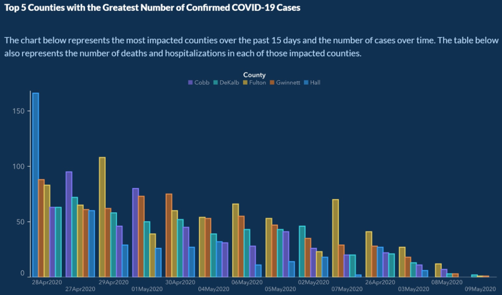
The power of graphic representation to make dense data more accessible has an embedded risk: Data in the wrong hands can be manipulative. This G eorgia Department of Public Health graphic , with its nonsensical ordering of days on the x-axis and its daily reordering of the counties to create a downward trend in the data, was particularly troubling.

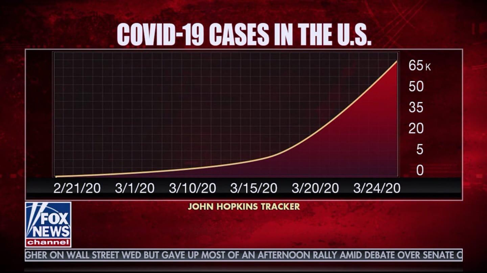
Another example is this graphic from Fox News , which uses different lengths between days on the x-axis and an inconsistent interval on the y-axis for the count of COVID-19 cases to reduce the slope of the line.

While it’s easy to see how these manipulated charts could sway a viewer’s judgment on the current risk of infection presented by COVID-19, Reinholtz, Maglio and Spiller examine how the format of a data visualization may impact a viewer’s judgment even when the information is appropriately presented and there is no intention of manipulating the viewer’s opinion.

Going with the Flow?

In an experiment, they found that participants’ interpretation of data — and their anticipated behavior based on that interpretation — was swayed by whether they saw a graphic showing the cumulative count of COVID-19 cases or one showing the trend line for daily new cases of infections.

The graphics below illustrate the difference in the two formats representing the same data from the CDC for the period between Jan. 22, 2020, and July 11, 2021. The left graphic shows daily new cases, a format known as “flow,” while the right graphic displays the cumulative number of cases, a format known as “stock.”

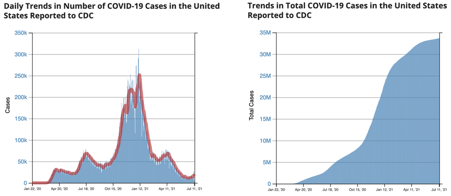
The cumulative graph on the right rises steeply when the left side showing daily cases rises. The cumulative graph then flattens as the daily cases return to lower levels. While it‘s possible to convert between the two formats, past research shows that even highly educated people have a difficult time doing so. In 2009, MIT graduate students were given the task to convert data between situations representing the two chart formats; fewer than one-third of the students made the conversions correctly.

For this reason, viewers usually interpret data based on the chart format presented to them. Reinholtz, Maglio and Spiller investigate whether viewers’ interpretation of the data is inconsistent when the trend of the graphs in the two formats moves in different directions. Since the cumulative number of COVID-19 cases is always increasing, divergence between the formats only happens when the daily number of new cases is decreasing. This diverging state occurs repeatedly over time as the number of new cases tends to rise and fall.

To examine this idea, the researchers conducted an experiment showing 20 days of COVID-19 data to 596 participants recruited online. The participants were first split into two groups; those who would be shown the data as a cumulative number of cases and those who would be shown the data as daily new cases of infections.

Both groups were further split with some shown one state’s data from March 16, 2020, to April 4, 2020, when the number of new cases was decreasing. And the rest were shown data from May 7, 2020, to May 26, 2020, when the number of new cases was increasing.

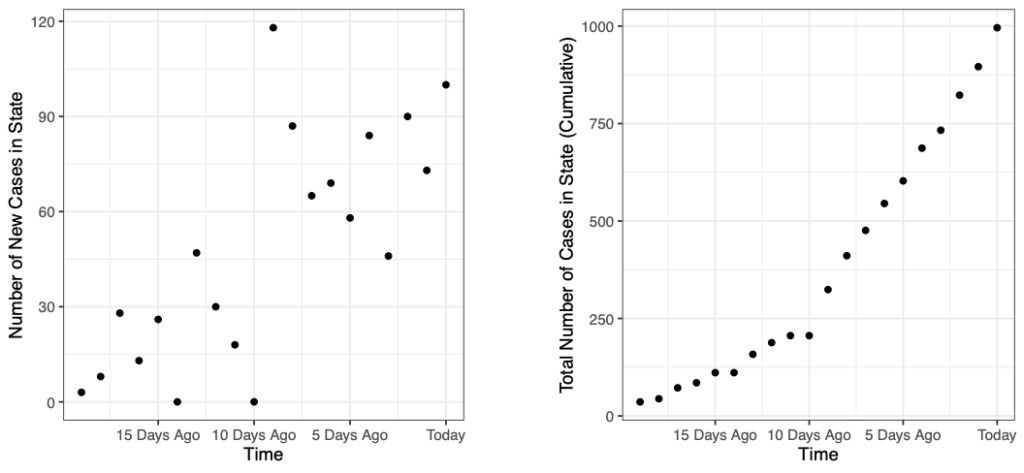
On the left side are the graphs of the daily changes in new COVID-19 infections, while the right side graphs the cumulative cases. The two graphs at the top represent the period when the number of new cases was increasing and the bottom two represent the period when the number of cases was decreasing.

After viewing their assigned graph, participants were asked to fill out a survey in which they indicated their opinion on the current level of risk and then were asked a series of questions to indicate how likely they would be to engage in certain behaviors given the level of risk. These questions included outdoor and indoor dining, using public transportation, having visitors in one’s home, sending their children back to school and various questions around shopping and using other services.

The researchers found that when daily new cases of COVID-19 were decreasing, participants perceived greater risk when viewing the data as cumulative cases of infections (showing an increasing trend) than when viewing the data as daily cases of new infections (showing a decreasing trend).

When daily cases were increasing there wasn’t much of a difference in judgments of risk as both charts showed an increasing trend. This was not a great surprise to the researchers given their past research in the area.

However, they were surprised to find that the participants’ behavioral intentions did not necessarily follow their risk judgments. Participants indicated a stronger intention to engage in risky behavior when they viewed a chart with the format as daily changes in new cases. They indicated a stronger likelihood to engage in risky behavior regardless of whether the trend of new cases was increasing or decreasing.

These findings suggest that what seems to be a minor choice in how to present data may lead to different conclusions about risk among viewers and even impact their intended behaviors. Based on these results, authorities may want to consider presenting data as cumulative cases, rather than daily changes, as a type of behavioral “nudge” to increase appropriate risk responses during a pandemic.

Featured Faculty

Associate Professor of Marketing and Behavioral Decision Making

About the Research

Reinholtz, N., Maglio, S. J., & Spiller, S. A. (in press). Stocks, Flows, and Risk Response to Pandemic Data . Journal of Experimental Psychology: Applied.

Suggested Articles

It’s a Startup — and Almost Certainly a Future Acquisition by a Tech Giant

Why Unloved Workers Don’t Share Productivity Tips with the Boss

Medical Debt in Collection Estimated at $140 Billion

Related articles.

The Dollar Store Fix for Vaccination Deserts

Pharmacies aren’t everywhere — adding dollar stores could reduce average distance to vaccination by 62%

Using Google Trends To Detect Revenue Misreporting

It’s public and free and could help auditors

Medicare Ratings Didn’t Predict Nursing Homes’ Initial COVID-19 Vulnerability

Rate of spread in the surrounding community was a bigger indicator of risk

Beyond Angry Mobs: Intellectuals in the French Revolution

History’s Encyclopédie subscribers are matched to grievances against the monarchy

Click through the PLOS taxonomy to find articles in your field.

For more information about PLOS Subject Areas, click here .

Loading metrics

Open Access

Peer-reviewed

Research Article

A statistical analysis of the novel coronavirus (COVID-19) in Italy and Spain

Roles Conceptualization, Data curation, Formal analysis, Investigation, Methodology, Project administration, Resources, Software, Validation, Visualization, Writing – original draft, Writing – review & editing

* E-mail: [email protected]

Affiliation School of Statistics, Renmin University of China, Beijing, China

• Jeffrey Chu

• Published: March 25, 2021
• https://doi.org/10.1371/journal.pone.0249037
• Reader Comments

The novel coronavirus (COVID-19) that was first reported at the end of 2019 has impacted almost every aspect of life as we know it. This paper focuses on the incidence of the disease in Italy and Spain—two of the first and most affected European countries. Using two simple mathematical epidemiological models—the Susceptible-Infectious-Recovered model and the log-linear regression model, we model the daily and cumulative incidence of COVID-19 in the two countries during the early stage of the outbreak, and compute estimates for basic measures of the infectiousness of the disease including the basic reproduction number, growth rate, and doubling time. Estimates of the basic reproduction number were found to be larger than 1 in both countries, with values being between 2 and 3 for Italy, and 2.5 and 4 for Spain. Estimates were also computed for the more dynamic effective reproduction number, which showed that since the first cases were confirmed in the respective countries the severity has generally been decreasing. The predictive ability of the log-linear regression model was found to give a better fit and simple estimates of the daily incidence for both countries were computed.

Citation: Chu J (2021) A statistical analysis of the novel coronavirus (COVID-19) in Italy and Spain. PLoS ONE 16(3): e0249037. https://doi.org/10.1371/journal.pone.0249037

Editor: Abdallah M. Samy, Faculty of Science, Ain Shams University (ASU), EGYPT

Received: July 14, 2020; Accepted: March 9, 2021; Published: March 25, 2021

Copyright: © 2021 Jeffrey Chu. This is an open access article distributed under the terms of the Creative Commons Attribution License , which permits unrestricted use, distribution, and reproduction in any medium, provided the original author and source are credited.

Data Availability: The raw data files for the incidence of COVID-19 in Italy and Spain are available from the following links: https://github.com/pcm-dpc/COVID-19 https://github.com/datadista/datasets/tree/master/COVID%2019 .

Funding: The author(s) received no specific funding for this work.

Competing interests: The authors have declared that no competing interests exist.

Introduction

The novel coronavirus (COVID-19) was widely reported to have first been detected in Wuhan (Hebei province, China) in December 2019. After the initial outbreak, COVID-19 continued to spread to all provinces in China and very quickly spread to other countries within and outside of Asia. At present, over 45 million cases of infected individuals have been confirmed in over 180 countries with in excess of 1 million deaths [ 1 ]. Although the foundations of this disease are very similar to the severe acute respiratory syndrome (SARS) virus that took hold of Asia in 2003, it is shown to spread much more easily and there currently exists no vaccine.

Since the first confirmed cases were reported in China, much of the literature has focused on the outbreak in China including the transmission of the disease, the risk factors of infection, and the biological properties of the virus—see for example key literature such as [ 2 – 6 ]. However, more recent literature has started to cover an increasing number of regions outside of China.

For example, studies covering the wider Asia region include: investigations into the outbreak on board the Diamond Princess cruise ship in Japan, using a Bayesian framework with a Hamiltonian Monte Carlo algorithm [ 7 ]; estimation of the ascertainment rate in Japan using a Poisson process [ 8 ]; modelling the evolution of the basic and effective reproduction numbers in South Korea using Susceptible-Infected-Susceptible models [ 9 ] and generalised growth models with varying growth rates [ 10 ]; modelling the basic reproduction number in India with a classical Susceptible-Exposed-Infectious-Recovered-type compartmental model [ 11 ]; forecasting numbers of cases in Indian states using deep learning-based models [ 12 ].

Analyses on North and South America have also used similar classical methods, for example [ 13 ] model the progression of the outbreak in the United States until the end of 2021 with the simple Susceptible-Infected-Recovered model, and [ 14 ] predict epidemic trends in Brazil and Peru using a logistic growth model and machine learning techniques. However, other studies include: analysis of the spatial variability of the incidence in the United States using spatial lag and error models, and geographically weighted regression [ 15 ]; estimation of the number of deaths in the United States using a modified logistic fault-dependent detection model [ 16 ]; estimating prevalence and infection rates across different states in the United States using a sample selection model [ 17 ]; investigating the relationship between social media communication and the incidence in Colombia using non-linear regression models.

Focusing on Africa, [ 18 ] simulate and predict the spread of the disease in South Africa, Egypt, Algeria, Nigeria, Senegal, and Kenya, using a modified Susceptible-Exposed-Infectious-Recovered model; [ 19 ] apply a six-compartmental model to model the transmission in South Africa; [ 20 ] predict the spread of the disease in West Africa using a deterministic Susceptible-Exposed-Infectious-Recovered model; [ 21 ] implement Autoregressive Integrated Moving Average models to forecast the prevalence of COVID-19 in East Africa; [ 22 ] predict the spread of the disease using travel history and personal contact in Nigeria through ordinary least squares regression; [ 23 ] use logistic growth and Susceptible-Infected-Recovered models to generate real-time forecasts of daily confirmed cases in Saudi Arabia.

Aside from many of the classical models mentioned above, recent developments in the econometrics and statistics literature have led to a number of new models that could potentially be applied in the modelling of infectious diseases. These include (but are not limited to) mixed frequency analysis, model selection and combination, and dynamic time warping. Mixed frequency analysis is an iterative approach proposed for dealing with the joint dynamics of time series data which are sampled at different frequencies [ 24 ]. In the economic literature, the common example is quarterly gross domestic product (GDP) and monthly inflation. [ 25 ] notes that studying the co-movements between mixed frequency data usually involves analysing the joint process sampled at a common low frequency, however, this can mis-specify the relationship. [ 24 , 25 ] propose vector autoregressive models for mixed frequency analysis that operate at the highest sampling frequency of all the time series in the model. These models allow for the modelling of the joint dynamics of the dependent and independent variables using time disaggregation, where the low frequency variables are interpolated and time-aggregated into a higher frequency. In the context of infectious diseases, such models could be beneficial for modelling the relationship between higher frequency data such as the number of daily cases or deaths and lower frequency data relating to, say, weekly cases or deaths, news and information about health prevention measures, etc. [ 26 , 27 ] propose the use of Bayesian Predictive Synthesis (BPS) for model selection and combination. They note that there are many scenarios that generate multiple, interrelated time series, where the dependence has a significant impact on decisions, policies, and their outcomes. In addition, methods need to learn and integrate information about forecasters and models, bias, etc. and how they change over time, to improve their accuracy [ 26 ]. Decision and policy makers often use multiple sources, models, and forecasters to generate forecasts, in particular, probabilistic density forecasts. However, although complex estimation methods may have useful properties for policy makers, large standard deviations may be a result of the complexity of the data, model, etc., and it may be difficult to know the source. The aim is to use the dependencies between time series to improve forecasts over multiple horizons for policy decisions [ 27 ]. For example, in the economic literature, setting interest rates based on utility or loss that account for inflation, real economy measures, employment, etc. BPS relates to a decision maker that accounts for multiple models as providers of “forecast data” to be used for prior-posterior updating. The decision maker learns over time about relationships between agents, forecasts, and dependencies, which are incorporated into the model, and dynamically calibrate, learn, and update weights for ranges of forecasts from dynamic models, with multiple lags and predictors [ 26 ]. In epidemiology, BPS could potentially be used in a similar context to analyse the dependency between various interrelated time series such as daily cases and deaths, hospital capacity, number vaccinations, etc. Different models and sources of data could then be combined and characterised in one single model improving the accuracy of forecasts. Dynamic time warping as noted by [ 28 , 29 ] is a technique that has not been widely used outside of speech and gesture recognition. It can be used to identify the relation structure between two time series by describing their non-linear alignment with warping paths [ 28 ]. The procedure involves a local cost measure characterising the sum of the differences between pairs of realisations of data at each time point, where an optimal warping path gives the lowest total cost. The optimal path is found under a variable lead-lag structure, where the most suitable lag can then be found [ 28 ]. This then reveals and identifies the lead-lag effects between the time series data. Indeed, dynamic time warping has recently been used in the modelling of COVID-19 by [ 30 ]. [ 30 ] use the method to determine the lead-lag relation between the cumulative number of daily cases of COVID-19 in various countries, in addition to forecasting the future incidence in selected countries. This allows for the classification of countries as being in the early, middle, and late stages of an outbreak.

Controlling an infectious disease such as COVID-19 is an important, time-critical but difficult issue. The health of the global population is, perhaps, the most important factor as research is directed towards vaccines and governments scramble to implement public health measures to reduce the spread of the disease. In most countries around the world, these measures have come in the form of local or national lockdowns where individuals are advised or required to remain at home unless they have good reason not to—e.g. for educational or medical purposes, or if they are unable to work from home. However, the implications of trying to control COVID-19 are being felt not only by the health sector, but also in areas such as the economy, environment, and society.

As the number of cases of infected individuals has risen rapidly, there has been an increase in pressure on medical services as healthcare providers seek to test and diagnose infected individuals, in addition to the normal load of medical services that are offered in general. In many cases, trying to control COVID-19 has led to a backlog for and deprivation of other medical procedures [ 31 ], with healthcare providers needing to find a balance between the two. [ 32 ] note that this conflict may change the nature of healthcare with public and private health sectors working together more often. The implementation of restrictions on the movement of individuals has also led to many suggesting that anxiety and distress may lead to increased psychiatric disorders. These may be related to suicidal behaviour and morbidity and may have a long-term negative impact on the mental health of individuals [ 33 , 34 ].

In addition to restrictions on the movement of individuals, governments have required most non-essential businesses to close. This has negatively impacted national economies with many businesses permanently closing leading to a significant increase in unemployment. Limits on travel have severely affected the tourism and travel industries, and countries and economies that are dependent on these for income. Whilst many of the implications of controlling COVID-19 on the economy are negative, there have been some positive changes as businesses adapt to the ‘new normal’. For example, the banking industry is dealing with increased credit risks, while the insurance industry is developing more digital products and pandemic-focused solutions [ 32 ]. The automotive industry is expected to see profits reduced by approximately $100 billion, which may be offset by the development of software subscription services of modern vehicles [ 32 ]. Some traditional office-based businesses have been able to reduce costs by shifting to remote working, while the restaurant industry has shifted towards takeaway and delivery services [ 32 ].

In terms of the environment, the limitations on businesses that have been able to continue operating throughout the epidemic has led to possible improvements in the environment—mainly from the reduction in pollution [ 35 ]. However, societal issues have been exacerbated. [ 32 ] note that the reduction in the labour force that has resulted from controlling for COVID-19 has affected ethnic minorities and women most significantly. Furthermore, in many countries health services employ more women than men creating a dilemma for working mothers—either leave the labour force and provide childcare for their families or remain in employment and pay extra costs for childcare.

In Europe, Italy and Spain were two of the first European countries to be significantly affected by COVID-19. However, the majority of the literature covering the two countries focuses on the clinical aspects of the disease, [ 36 – 40 ], with only a limited number exploring the prevalence of the disease, [ 41 – 43 ].

As as a result of this on going pandemic, new results and reports are being produced and published daily. Thus, our motivation stems from wanting to contribute to the statistical analysis of the incidence of COVID-19 in Italy and Spain, where the literature is limited. The main contributions of this paper are: i) to model the incidence of COVID-19 in Italy and Spain using simple mathematical models in epidemiology; ii) to provide estimates of basic measures of the infectiousness and severity of COVID-19 in Italy and Spain; iii) to investigate the predictive ability of simple mathematical models and provide simple forecasts for the future incidence of COVID-19 in Italy and Spain.

The contents of this paper are organised as follows. In the data section, we describe the incidence data used in the main analysis and provide a brief summary analysis. The method section outlines the Susceptible-Infectious-Recovered model and the log-linear model used to model the incidence of COVID-19, and introduces the basic reproduction number and effective reproduction number as measures of the infectiousness of diseases. In the results section, we present the main results for the fitted models and estimates of the measures of infectiousness, in addition to simple predictions for the future incidence of COVID-19. Some concluding remarks are given in the conclusion.

The data used in this analysis consists of the daily and cumulative incidence (confirmed cases) of COVID-19 for Italy and Spain (nationally), and their respective regions or autonomous provinces. For Italy, this data covers 21 regions for 37 days from 21st February 2020 to 28th March 2020, inclusive; for Spain, this data covers 19 regions for 34 days from 27th February to 31st March 2020, inclusive. The data for Italy was obtained from [ 44 ] where the raw data was sourced from the Italian Department of Civil Protection; the data for Spain was obtained from [ 45 ] where the raw data was sourced from the Spanish Ministry of Health. The starting dates for both sets of data indicate the dates on which the first cases were confirmed in each country, however, it should be noted that in some regions cases were not confirmed until after these dates. These particular time periods were chosen as they cover over one month since the initial outbreaks in both countries and were the most up to date data available at the time of writing. In the remainder of this section, we provide a simple exploratory analysis of the incidence data.

Fig 1 plots the daily cumulative incidence for Italy and its 21 regions over the whole sample period. All cumulative incidence appears to show an exponential trend, increasing slowly for the first 14 days after the first cases are confirmed before growing rapidly. Checking the same plot on a log-linear scale, shown in Fig 2 , we find that the logarithm of cumulative incidence in some regions exhibits an approximate linear trend suggesting that cumulative incidence is growing exponentially. However, in the majority of regions (and nationally) this trend is not exactly linear, suggesting a slightly sub-exponential growth in cumulative incidence.

• PPT PowerPoint slide
• PNG larger image
• TIFF original image

https://doi.org/10.1371/journal.pone.0249037.g001

https://doi.org/10.1371/journal.pone.0249037.g002

Of all the regions in Italy, the northern region of Lombardy is one of the worst affected and Fig 3 plots the daily incremental incidence for both Lombardy and Italy, respectively. In terms of the number of new cases confirmed each day, the trends are very similar and, again, possibly exponential until peaking around 21st March 2020 before levelling off. Comparing the trends for the other regions in Fig 4 , it can be seen that other significantly affected northern regions such as Piedmont and Emilia-Romagna exhibit similarities to Lombardy—growing, peaking, and levelling around the same times. However, many other regions show some slight differences such as peaking at earlier or later dates, and even exhibiting an erratic trend.

https://doi.org/10.1371/journal.pone.0249037.g003

https://doi.org/10.1371/journal.pone.0249037.g004

In Fig 5 , things are put in perspective when the cumulative incidence of all Italian regions are plotted on the same scale. It is clear that Lombardy is the most affected region contributing to the largest share of national cumulative incidence, and indeed it is the epicentre of the outbreak in Italy.

https://doi.org/10.1371/journal.pone.0249037.g005

In the case of Spain, Fig 6 plots the daily cumulative incidence nationally and for all 19 Spanish regions over the whole sample period. The trend appears to be exponential and is similar between regions, but is also similar to that of the daily cumulative incidence in Italy. On a log-linear scale, in Fig 7 , the growth of the daily cumulative incidence appears to be closer to an exponential trend compared with Italy, due to the plots arguably exhibiting a more linear trend. It can be seen that there is a slight difference with Italy in that it appears as though most Spanish regions were affected at approximately the same time—when the country’s first cases were confirmed. This is reflected by the majority of plots starting from the very left of the x-axis, with the exception of the plots for a few regions such as Ceuta and Melilla. In Italy only a small number of regions were affected when the country’s first cases were confirmed, with the growth in cumulative incidence for the majority of the other regions coming later on.

https://doi.org/10.1371/journal.pone.0249037.g006

https://doi.org/10.1371/journal.pone.0249037.g007

The worst affected regions in Spain are Madrid and Catalonia, and Fig 8 plots the daily incremental incidence for both regions and the national trend. The growth in daily incidence, in all three cases, could be classed as being approximately exponential, however, daily incidence appears to peak on 26th March 2020 before falling and peaking again on 31st March 2020. It is confirmed that the true peak daily incidence does indeed occur on 31st March 2020 and we return to this point later on in the analysis. In comparison to other Spanish regions, it seems that Madrid and Catalonia are the exceptions as the majority of regions exhibit an exponential rise in daily incidence and peak around 26th and 27th March 2020 before falling.

https://doi.org/10.1371/journal.pone.0249037.g008

Plotting the daily incidence of all regions on the same scale in Fig 9 , it is clear that Madrid and Catalonia are the most affected regions contributing the largest share of the national cumulative incidence. Whilst Madrid and Catalonia are the main epicentres of the outbreak in Spain, many coastal regions also show significant numbers of confirmed cases, although not quite on the same scale.

https://doi.org/10.1371/journal.pone.0249037.g009

The SIR (Susceptible-Infectious-Recovered) model

In the mathematical modelling of infectious diseases, there exist many compartmental models that can be used to describe the spread of a disease within a population. One of the simplest models is the SIR (Susceptible-Infectious-Recovered) model proposed by [ 46 ], in which the population is split into three groups or compartments: those who are susceptible ( S ) but not yet infected with the disease; those who are infectious ( I ); those who have recovered ( R ) and are immune to the disease or who have deceased.

The SIR model has been extensively researched and applied in practice, thus it would not be practical to mention and cover all of the literature. However, some of the most prominent literature covers areas such as the stability and optimality of the simple SIR model ([ 47 – 51 ]); pulse vaccination strategy in the SIR model ([ 52 – 55 ]); applications of the SIR in the modelling of infectious diseases ([ 56 – 64 ]).

With regards to COVID-19, many have applied the basic SIR model (or slightly modified versions) to model the outbreak. Some particular examples include (but are not limited to): [ 2 ] who estimate the overall symptomatic case fatality risk of COVID-19 in Wuhan and use the SIR model to generate simulations of the COVID-19 outbreak in Wuhan; [ 65 ] who apply a modified SIR model to identify contagion, recovery, and death rates of COVID-19 in Italy; [ 66 ] who combine the SIR model with probabilistic and statistical methods to estimate the true number of infected individuals in France; [ 67 ] who use a number of methods including the SIR model to estimate the basic and controlled reproduction numbers for the COVID-19 outbreak in Wuhan, China; [ 68 ] who show that the basic SIR model performs better than extended versions in modelling confirmed cases of COVID-19 and present predictions for cases after the lockdown of Wuhan, China; [ 69 ] who model the temporal dynamics of COVID-19 in China, Italy, and France, and find that although the rate of recovery appears to be similar in the three countries, infection and death rates are more variable; [ 70 ] who simulate the outbreak in Wuhan, China, using an extended SIR model and investigate the age distribution of cases; [ 71 ] who study the number of infections and deaths from COVID-19 in Sweden using the SIR model; [ 72 ] who use the SIR model, with an additional parameter for social distancing, to model and forecast the early stages of the COVID-19 outbreak in Brazil.

In reference to the SIR model, [ 74 ] note that it “examines only the temporal dynamics of the infection cycle and should thus be appropriate for the description of a well-localised epidemic outburst”, therefore, it would appear to be reasonable for use in analysis at city, province, or country level. In the form above, the dynamics of the model are controlled by the parameters β and γ , representing the rates of transition from S to I (susceptibility to infection), and I to R (infection to recovery or death), respectively.

To fit the model and find the optimal parameter values of β and γ , we use the optim function in R [ 75 ] to solve the minimisation problem. The system of differential equations, Eqs ( 1 ) to ( 3 ), are set up as a single function. The model is then initialised with starting values for S , I , and R , with parameters β and γ unknown. We obtain the daily cumulative incidence for the sample period, total population ( N ), and the susceptible population ( S ) as the total population minus the number of currently infected individuals. This is defined as the cumulative number of infected individuals minus the number of recovered or dead, however, these exact values are difficult to obtain. Thus, the cumulative number of infected individuals at the start date of the sample period is used as a proxy—since at the start date of the disease, this is likely to be close to the true value, as the number of recovered or dead should be very small (if not zero).

The residual sum of squares is then defined and set up as a function of β and γ . The optim package is used for general purpose optimisation problems, and in this case it is used to minimise the function RSS with respect to the sample of cumulative incidence. More specifically, we use the limited memory Broyden-Fletcher-Goldfarb-Shanno (L-BFGS-B) algorithm for the minimisation, which allows us to specify box constraints (lower and upper bounds) for the unknown parameters β and γ . The lower and upper bounds of zero and one, respectively, were selected for both parameters. The optim function then searches for the β and γ that minimise the RSS function, given starting values of 0.5 for both parameters. The optimal solution is found via the gradient method by repeatedly improving the estimates of RSS to try and find a solution with a lower value. The function makes small changes to the parameters in the direction of where RSS changes the fastest, where in this direction the lowest value of RSS is. This is repeated until no further improvement can be made or the improvement is below a threshold.

We consider convergence as the main criteria for finding an optimal solution in the minimisation of RSS —when the lowest RSS has been found, and no further improvement can be found or the improvement is below a threshold. In the case where convergence is not achieved, or there is some related error, then we use the parscale function in the optimisation. As the true values of β and γ are unknown, in the default case, the parameters are adjusted by a fixed step starting from their initial values. Most common issues were addressed using the parscale function to rescale—alter the sensitivity/magnitude of the parameters on the objective function. In other words, it allows the algorithm to compute the gradient at a finer scale (similar to the ndeps parameter—used to adjust step sizes for the finite-difference approximation to the gradient). In most cases, issues were solved by using a step size of 10 −4 . Of course, smaller step sizes could be used, but there is a risk that selecting too small a step size will lead to the optimal values of β and γ being found at their starting values. However, the results should be interpreted with caution. It is possible that estimates will vary with different population sizes N and the starting values specified for β and γ , which may also cause the optimisation process to be unstable.

It should be noted that the application of the basic SIR model to COVID-19 simplifies the analysis and makes the strong assumption that individuals who become infected but recover are immune to COVID-19. This is assumed purely for the simplification of modelling and we do not claim this to be true in reality. At present, it remains unclear whether those who recover from infection are immune [ 76 ]. Indeed, there have been studies and unconfirmed reports of individuals who have possibly recovered but then subsequently tested positive for the virus again, see for example [ 77 – 79 ].

The basic reproduction number R 0

Whilst the fitted model and optimal parameters allow us to make a simple prediction about how the trajectory of the number of susceptible, infectious, and recovered individuals evolves over time, a more useful statistic or parameter that can be computed from the fitted model is the basic reproduction number R 0 . Originally developed for the study of demographics in the early 20th century, it was adapted for use in the study of infectious diseases in the 1950’s [ 80 ]. It is defined as the “expected number of secondary infections arising from a single individual during his or her entire infectious period, in a population of susceptibles” [ 80 ], and is widely considered to be a fundamental concept in the study of epidemiology. In other words, it is the estimated number of people that an individual will go on to infect after becoming infected.

The R 0 value can provide an indication of the severity of the outbreak of an infectious disease: if R 0 < 1, each infected individual will go on to infect less than one individual (on average) and the disease will die out; if R 0 = 1, each infected individual will go on to infect one individual (on average) and the disease will continue to spread but will be stable; if R 0 > 1, each infected individual will go on to infect more than one individual (on average) and the disease will continue to spread and grow, with the possibility of becoming a pandemic ([ 80 , 81 ]).

Log-linear model

https://doi.org/10.1371/journal.pone.0249037.g010

To fit the log-linear model, we use the incidence package [ 82 ] in R [ 75 ] to obtain the optimal values of the parameters. Using the estimated parameters, the fitted model can be used to predict the trajectory of the incidence up until the peak incidence in the growth phase. However, although the log-linear model allows for the modelling and prediction of the incidence, compared with the SIR model it does not provide any indication about the number of susceptible or recovered individuals.

We are able to use the epitrix R package [ 84 ] to implement the method by [ 83 ] for empirical distributions to estimate R 0 from the growth rate r . However, [ 83 ] note that an “epidemic model implicitly specifies a generation interval distribution” (also known as the serial interval distribution), which is defined as “the time between the onset of symptoms in a primary case and the onset of symptoms in secondary cases” [ 85 ]. As we do not have access to more detailed COVID-19 patient data, we are not able to compute the parameters of the serial interval distribution directly. However, a number of existing analyses of COVID-19 patient data report some preliminary estimates of the best fitting serial interval distributions and their corresponding model parameters. These are: i) gamma distribution with mean μ = 7.5 and standard deviation σ = 3.4 [ 81 ]; ii) gamma distribution with mean μ = 7 and standard deviation σ = 4.5 [ 2 ]; iii) gamma distribution with mean μ = 6.3 and standard deviation σ = 4.2 [ 86 ]. By using these three serial intervals in conjunction with the above method, we are able to obtain estimates of R 0 from estimates of the growth rate r . It should be noted that serial interval distributions are not only restricted to the gamma distribution—other common distributions used include the Weibull and log-normal distributions, and that the parameters are dependent on a number of factors including the time to isolation [ 86 ].

The effective reproduction number R e

As mentioned above, the estimation of the R 0 value is not always ideal, due to it being a single fixed value reflecting a specific period of growth (in the log-linear model) or requiring assumptions that only hold true in specific time periods (in the basic SIR model). In other words, it is “time and situation specific” [ 85 ]. In reality, the reproduction number will vary over time but it will also be influenced by governments and health authorities implementing measures in order to reduce the impact of the disease. Therefore, a more useful approach for measuring the severity of an infectious disease is to track the reproduction number over time. The effective reproduction number R e is one way to achieve this, and thus allows us to see how the reproduction number changes over time in response to the development of the disease itself but also effectiveness of interventions. Although there are numerous methods that can be used to analyse the severity of a disease over time, the majority are not straightforward to implement (especially in software) [ 85 ].

One popular method for estimating R e is that proposed by [ 85 ]. The basic premise of this method is that “once infected, individuals have an infectivity profile given by a probability distribution w s , dependent on time since infection of the case, s , but independent of calendar time, t . For example, an individual will be most infectious at time s when w s is the largest. The distribution w s typically depends on individual biological factors such as pathogen shedding or symptom severity” [ 85 ].

The function models the transmissibility of a disease with a Poisson process, such that an individual infected at time t − s will generate new infections at time t at a rate of R t w s , where R t is the instantaneous (effective) reproduction number at time t . Thus, the incidence at time t is defined to be Poisson distributed with mean equal to the average daily incidence (number of new cases) at time t . This value is just for a single time period t , however, estimates for a single time period can be highly variable meaning that it is not easy to interpret, especially for making policy decisions. Therefore, we consider longer time periods of one week (seven days)—assuming that within a rolling window the instantaneous reproduction number remains constant. Note that there is a potential trade off, as using longer rolling windows gives more precise estimates of R t but this means fewer estimates can be computed (requires more incidence values to start with) and a more delayed trend reducing the ability to detect changes in transmissibility. Whereas shorter rolling windows lead to more rapid detection in changes but with more noise. Using this method, it is recommended that a minimum cumulative daily incidence of 12 cases have been observed before attempting to estimate R e . For the data sets used, this does not pose a problem as a cumulative total of 16 and 17 cases, respectively, exist on the first day of the sample at the country level, and by the seventh day the totals are around 200 and 650 for Spain and Italy, respectively.

From the posterior distribution, the posterior mean R t , τ can be computed at time t for the rolling window of [ t − τ , t ] by the ratio of the gamma distribution parameters. We refer the readers to the supplementary information of [ 85 ] for further details regarding the Bayesian framework. As noted by [ 85 ], this method works best when times of infection are known and the infectivity profile or distribution can be estimated from patient level data. However, as mentioned above, we do not have access to this level of data, and instead utilise three different serial intervals from the literature that have been estimated from real data.

In practice, the transmission of a disease will vary over time especially when health prevention measures are implemented. However, this method is the only reproduction number that can be easily computed in real-time, and in comparison to similar methods, it captures the effect of control measures since it will cause sudden decreases in estimates compared with other methods.

In this analysis, we use the most basic version of this method and estimate the effective reproduction number over a rolling window of seven days. This appears to be sufficient and in line with our results, as we do not suffer from the problem of small sample sizes as the samples are sufficiently large and we start computing the effective reproduction number after one mean serial interval. It should be noted that estimates of this reproduction number are dependent on the distribution of the infectiousness profile w s . In addition, it is known that this distribution may not always be well documented, especially in the early parts of an epidemic. However, here we assume that the serial interval is defined for our sample period and the use of the three serial intervals from the literature appears to give satisfactory results.

If problems did arise, or to account for uncertainty in the serial interval distribution, an alternative method is to implement a modified procedure by [ 85 ], which allows for uncertainty in the serial interval distribution. This modified method assumes that the serial interval is gamma distributed but the mean and standard deviation are allowed to vary according to a standard normal distribution. Some N * pairs of means and standard deviations are simulated—mean first and standard deviation second, with the constraint that the mean is less than the standard deviation to ensure that for each pair the probability density function of the serial interval distribution is null at time t = 0. Then, for each rolling window 1000 realisations are sampled of the instantaneous reproduction number using the posterior distribution conditional on the pair of parameters.

The SIR model and R 0

For both Italy and Spain, we set up and solve the minimisation problem for the SIR model described in Section for region-level and national-level COVID-19 incidence for the first 14 days after the first cases were confirmed in each respective country and region. The first 14 days after the first cases are detected can be considered to be the early stage of an outbreak, and it is reasonable to assume that there are few, if no, infected or immune individuals prior to this. However, it is a rather strong assumption as it is possible that individuals may be infected but do not display any symptoms. Tables 1 and 2 show the output corresponding to each region/country including the date that the first cases were confirmed, the population size (obtained from [ 88 ]), the cumulative number of cases at the 14th day after the first cases were confirmed, the fitted estimates for the parameters β and γ , and estimates for R 0 .

https://doi.org/10.1371/journal.pone.0249037.t001

https://doi.org/10.1371/journal.pone.0249037.t002

From Tables 1 and 2 , we observe that many of the first regions to be affected in both countries are those with the largest population sizes, however, the cumulative number of cases (after the first 14 days) in these regions are not always the highest among all regions. The estimates of the parameters β and γ also do not show any particular trends and this is reflected in the estimated R 0 values. It can be seen that for all regions in both Italy and Spain, the estimated R 0 values fall between one and three. This suggests that, according to the thresholds described above, the disease is spreading and growing in all Italian and Spanish regions during the 14 days after the first localised cases were confirmed. At a national level, the estimated values of R 0 are greater than two for both countries, again, suggesting a spreading and growing disease. This is perhaps not surprising since this time period reflects the early stages of the spread of the disease, thus we would expect it to be growing and spreading quickly before any preventative action is taken.

We note that in Tables 1 and 2 , there are some cases where the estimated value of β is very close to or at the upper limit of 1.000—e.g. Lombardy (Italy) and Madrid (Spain). This leads to the consequence that the parameter estimates appear to be bound by the upper limit. However, all parameter estimates are dependent on the starting values defined for β and γ , and the upper and lower bounds specified. For all cases of estimating the parameters in Tables 1 and 2 , we used the same optimisation procedure and criteria for determining a satisfactory estimate that is the convergence in the minimisation of the RSS ( Eq (4) ). In all cases, convergence was achieved but this is still slightly problematic. For cases where the estimated value of β is 1.000, although convergence was achieved, this indicates only that it generates the lowest RSS within the upper and lower limits defined. Therefore, there may or may not exist values of the parameter outside of this range that may be more optimal. Indeed, the results may vary depending on the upper and lower bounds, and the starting values that are selected. Thus, there is also the question of how to change the starting values and bounds appropriately (instead of, say, simply increasing them). Furthermore, as the R 0 value in the SIR model is computed as β / γ , another consequence of the estimated value of β being 1.000 is that the true value of β may actually be larger than this, and so the true value of R 0 may be larger than the estimated value.

Using the estimated parameters for the best fitted models, the predicted trajectories of the numbers in each of the compartments of the model can be generated. For brevity, in the remainder of the analysis, we show only the results for Italy, Spain, and their worst affected regions. Fig 11 plots the observed and predicted cumulative incidence for the 14 days immediately following the first confirmed cases in Lombardy and Italy, respectively. It can be seen that the model appears to under predict the true total number of cases in both cases during the early part of the outbreak before over estimating towards the end of the 14 days. In Fig 12 the SIR model trajectories are plotted along with the observed cumulative incidence on a logarithmic scale for Lombardy and Italy. The under prediction of the cumulative incidence in the first 14 days (to the left of the vertical dashed black line) is indicated by the solid red line (predicted cumulative incidence) lying below the black points (observed cumulative incidence) however, after the initial 14 days and after the implementation of a nationwide lock down (vertical dashed red line), the observed cumulative incidence grows at a slower rate than predicted by the fitted model. Indeed, this reflects the fact that the model is based only on the initial 14 days and does not account for any interventions.

https://doi.org/10.1371/journal.pone.0249037.g011

https://doi.org/10.1371/journal.pone.0249037.g012

In Fig 13 , the observed and predicted cumulative incidence for the 14 days immediately following the first confirmed cases in Catalonia, Madrid, and Italy, respectively, are shown. In contrast to the results for Italy, the fitted model for all three appears to predict the true total number of cases across the whole of the first 14 days reasonably well. Fig 14 plots the SIR model trajectories and the observed cumulative incidence on a logarithmic scale for Catalonia, Madrid, and Spain. Here, the more accurate predictions of the cumulative incidence are reflected in the area to the left of the vertical dashed black line. However, it can be seen that at the time when the nationwide lock down came into force (vertical dashed red line) the growth of the true total number of cases slowed down. It is likely that this is coincidental, since it is known that the effect on the incidence of infectious diseases from health interventions is not immediate, but instead lags behind.

https://doi.org/10.1371/journal.pone.0249037.g013

https://doi.org/10.1371/journal.pone.0249037.g014

Log-linear model and R 0

Following the SIR model, we implemented the log-linear model as described above for region-level and national-level COVID-19 daily incidence for the entire growth phase (from the time of the first confirmed cases until the time at which daily incidence peaks). The estimated parameters of the fitted log-linear models for the daily incidence of Lombardy and Italy, respectively, are shown in Table 3 . It can be seen that the peak daily incidence in both Lombardy and at country level occurred on the same day (21st March 2020), however, the growth rate (doubling time) is found to be slightly greater (shorter) at country level (0.18 and 3.88) compared with the Lombardy region (0.16 and 4.34). In comparison to the SIR model and modelling the cumulative incidence, the log-linear model modelling the daily incidence in the growth phase (as shown in Fig 15 ) appears to be slightly more accurate.

Upper and lower limits of the 95% confidence intervals are indicated by the dashed red lines.

https://doi.org/10.1371/journal.pone.0249037.g015

https://doi.org/10.1371/journal.pone.0249037.t003

In Table 4 , the estimated parameters of the fitted log-linear models for the daily incidence of Madrid, Catalonia, and Spain, respectively, are given. Similarly, the peak daily incidence occurs on the same day (31st March 2020) for Madrid, Catalonia, and Spain, although this is later than that for Italy. Interestingly, the growth rate (doubling time) is greatest (shortest) for Catalonia (0.24 and 3.85), whilst Madrid and Spain share similar growth rates and doubling times (0.21/0.22 and 3.24/3.21). It should be noted that there appears to be a slight difference in the observed daily incidence compared with the case of Italy and its regions. In Fig 16 , it can be seen that the observed daily incidence appears to initially peak in the last few days of March in all cases before falling, but then increases to a higher peak at the end of the growth phase. This seems to throw off the fitted log-linear model, as after the initial (approximate) 14 days the fitted model under predicts and then over predicts the daily incidence.

https://doi.org/10.1371/journal.pone.0249037.g016

https://doi.org/10.1371/journal.pone.0249037.t004

As with the SIR model, we are also able to use the fitted log-linear models in conjunction with the three serial intervals mentioned above to compute estimates of the R 0 value. Table 5 shows the mean estimates of the R 0 value for Italy, Spain, and their most affected regions, computed from the fitted log-linear models and the three serial intervals. In each case, the mean estimates are computed from 10,000 samples of R 0 values generated from the log-linear regression of the incidence data in the growth phase, and the distributions of these samples are plotted in S1 Fig . Compared with the estimates from the SIR model, we find that in all but the case of Italy, the estimates of R 0 from the log-linear model are greater than that from the SIR model—in these cases, the lowest estimates of R 0 from the log-linear models are larger by between 0.5 to 1. In the case of Italy, we find that the estimate of R 0 computed from the SIR model is approximately the same as that computed from the log-linear model using a serial interval using a gamma distribution with mean μ = 7 and standard deviation σ = 4.5 [ 2 ]. Using the log-linear models, the largest R 0 values computed are for Catalonia, whereas the smallest values are for Lombardy. It can also be seen that serial distributions with a lower mean appear to correspond with lower R 0 values. A possible explanation for the difference between the estimated R 0 values computed from the SIR models and the log-linear models is that the only incidence data from the first 14 days was used in the former, whereas incidence data from the whole growth phase was used in the latter—almost double the data. Therefore, it is arguable that the R 0 estimates from the log-linear models could be considered to be more accurate.

https://doi.org/10.1371/journal.pone.0249037.t005

Effective reproductive number R e .

Turning towards the more dynamic measure of the infectiousness of diseases, Figs 17 and 18 plot the estimated reproductive numbers computed for Lombardy, Italy, Madrid, Catalonia, and Spain, over the entire sample period. Using the method proposed by [ 85 ], in each case estimates were computed using rolling windows of the daily incidence over the previous 7 days and the same three serial distributions as for the log-linear models. As a result, no estimates are computed for the first 7 days of each respective sample period. In all cases, we analyse and compute the R e values over the whole sample period available allowing us to see how the infectiousness of COVID-19 varies during the initial outbreak stages and the effect of any interventions implemented by the respective governments. In Fig 17 , we observe that for both Lombardy and Italy, R e is generally decreasing over the time (under any of the three serial distributions), and although it is initially larger for Italy, after approximately the first 7 days the R e values are similar. However, the trend of R e both to the left and right (before and after) of the nationwide lockdown (indicated by the dotted line) shows some differences. Prior to the nationwide lockdown, R e decreases rapidly towards a value of between three and four, which could be attributed to the fact that northern Italy (including Lombardy) was the most affected area in the early stages of the outbreak and lockdowns local to the area were already being enforced from 21st February 2020. Thus, this is likely to have contributed (in part) to the initial reduction in the R e value. After the nationwide lockdown came into force on 9th March 2020, R e continues to decrease but at a slower pace and appears to level off approximately 14 days later—this coincides with the peak in daily incidence on 21st March 2020. After this point, it is likely that the effects of the nationwide lockdown are starting to appear with R e appearing to decrease again more rapidly towards the critical value of one (solid horizontal line)—suggesting that the disease is still spreading but stabilising.

Upper and lower limits of the 95% confidence intervals for the mean are indicated by the red dashed lines, and the grey dotted line indicates the date at which the national lock down becomes effective.

https://doi.org/10.1371/journal.pone.0249037.g017

https://doi.org/10.1371/journal.pone.0249037.g018

In Fig 18 , we observe a different trend in the R e value for Madrid, Catalonia, and Spain, compared with Lombardy and Italy. Whilst R e exhibits a decrease over the sample time period (under any of the three serial distributions), the initial values are actually larger for Madrid and Catalonia, however, the values for all three are similar after the initial 7 days. The trend in the estimated R e values before and after the nationwide lockdown again show some differences, but also differ to those for the cases of Lombardy and Italy. Prior to the nationwide lockdown (indicated by the dotted line), the trend of the estimated R e values is very erratic: decreasing, increasing, and then decreasing again. This could be due to the daily incidence for Madrid, Catalonia, and Spain, showing greater variation compared with that for Italy before the respective lockdowns. It is found that in the period before the lockdowns, Spanish daily incidence appears to show more alternation between increases and decreases compared with the previous day’s incidence, whilst Italian daily incidence shows much less. After the nationwide lockdown on 14th March 2020, for all three cases the estimated R e decreases significantly towards a value of two. More specifically, in mid-March 2020 daily incidence for Madrid, Catalonia, and Spain, levels off corresponding to the reduction in R e , but in the run up to 23rd March 2020 daily incidence again becomes more variable and alternates between significantly larger and smaller daily incidence, with R e levelling off. After 23rd March 2020, this levelling off is more sustained for Madrid and Spain compared with Catalonia. This may be attributed to the daily incidence initially peaking and then decreasing much more significantly for Catalonia, leading to a more significant decrease in R e at the latter end of the sample period. In general, the estimated R e values are larger for Spain than Italy, since Spain is lagging behind in terms of the start of the outbreak, however, it is found that the estimated R e is larger for Italy than Spain, but larger for Madrid and Catalonia than Lombardy.

Predictive ability of models.

Whilst the results regarding the estimated reproduction values ( R 0 and R e ) provide useful indicators about the infectiousness of COVID-19 and the variability over time, the predictive ability of models is also key—especially in the decay phase of an outbreak after the daily incidence has peaked and is in decline. Predictions about the daily incidence in the decay phase can contribute to determining whether health interventions are working, but can additionally provide time frames for when daily incidence may reach certain thresholds—e.g. below which the disease may be considered under control. To compare the predictive ability of the SIR and log-linear models, we use the projections package [ 89 ] in R [ 75 ]. As this section acts to provide only a brief analysis of the predictive ability of the models, we refer the readers to [ 89 ] for in-depth documentation regarding the finer details of the computations. The initial step is to consider which of the two models provides the best predictive ability in the growth phase of the COVID-19 outbreak and for simplicity, we analyse only Italy and Spain at country level. Using the estimated R 0 values for Italy and Spain from the SIR and log-linear models above, we combine these with the three serial distributions mentioned earlier. We then use the projections package [ 89 ] to forecast and predict the daily incidence for Italy and Spain from the 14th day (since the first cases in each location) until the day of peak incidence.

Plots of the true daily incidence in Italy and Spain during their respective growth phases and the predicted values using the SIR and log-linear models are shown in Figs 19 and 20 . In each figure, the first row plots the predictions using the SIR model; the second row plots the predictions using the log-linear model. For the case of Italy, the plots in Fig 19 appear to show that the predictions using the R 0 value estimated from the SIR model and the serial interval of a gamma distribution with mean μ = 7.5 and standard deviation σ = 3.4 [ 81 ] provide the most accurate general predictions. However, although using the R 0 value estimated from the log-linear model generates predictions which are accurate up until the last 7 days of the growth phase (where all three cases show over prediction), these results are more consistent compared with those using the SIR model. For the case of Spain, the plots in Fig 20 show that the predictions using the R 0 value estimated from the SIR model are consistent but significantly under predicting the observed daily incidence. In contrast, predictions using the R 0 value estimated from the log-linear model are consistent and accurate up until the initial peak in daily incidence a few days before the true peak at the end of the growth phase. Based on these results for the growth phase of the outbreak, we propose to use the log-linear model to compute basic predictions for the decay phase.

95% confidence intervals for the predicted incidence are indicated by the shaded light purple regions.

https://doi.org/10.1371/journal.pone.0249037.g019

https://doi.org/10.1371/journal.pone.0249037.g020

At the time of conducting this part of the analysis, approximately one month of daily incidence data was available for the decay phase (following peak daily incidence) of both Italy and Spain. Similarly, we follow the methodology for fitting the log-linear model but now apply it to the decay phase daily incidence. The model is fitted to the decay phase daily incidence in the same way, and model parameters can be computed. Note that for the decay phase, the values and interpretation of the estimated parameters change—the growth rate takes a negative value and the doubling time becomes the halving time (both reflecting the decay and decrease in daily incidence). The fitted log-linear regressions for Italy and Spain are shown in the left hand plots of Figs 21 and 22 , respectively. The fitted models appear to provide reasonable fits to the observed decay phase daily incidence much like the case for the growth phase.

Plots of the observed (dot-dashed black line) and projected daily incidence for the next 180 days using the log-linear model and serial interval distributions SI 1 (green line), SI 2 (blue line), and SI 3 (red line) (right).

https://doi.org/10.1371/journal.pone.0249037.g021

https://doi.org/10.1371/journal.pone.0249037.g022

Also, as in the growth phase, the R 0 value can still be computed for the log-linear model during the decay phase, and for consistency we obtain mean estimates of R 0 from 10,000 samples of R 0 generated from the log-linear regressions of the daily incidence during the decay phase in conjunction with the three serial distributions. Distributions of these estimates are plotted in S2 Fig and it can be seen that (in contrast to the growth phase) the mean estimates of R 0 for Italy and Spain, individually, are very similar (under the three serial distributions)—between 0.85 and 0.87 for Italy, and 0.77 and 0.83 for Spain. Using the mean estimated R 0 values and the three serial distributions, we computed projections of the daily incidence for the 180 days immediately following the end of the decay phase sample period on 22nd April 2020. The paths of these projections for Italy and Spain are shown in the right hand plots of Figs 21 and 22 , respectively.

A simple comparison of the projected daily incidence for both countries is given in Table 6 , at one and two months following the end of the decay phase sample period. Observed daily incidence for the remainder of the decay phase was obtained from [ 44 , 90 , 91 ]. In general, it appears that the predictions for future daily incidence (under all three serial distributions) in both Italy and Spain are significantly greater than the observed daily incidence. At the one month time point (21st May 2020) projections of daily incidence for Italy are approximately twice as large as the true incidence; projections of daily incidence for Spain are approximately two to three times as large as the true incidence. Moving forward to the two month time point (21st June 2020) projections of the daily incidence for Italy are approximately two to three times as large as the true incidence; projections of the daily incidence for Spain are up to twice as large as the true incidence. However, the projection of Spanish daily incidence using the serial interval of a gamma distribution with mean μ = 6.3 and standard deviation σ = 4.2 [ 86 ] is almost identical to the true incidence.

https://doi.org/10.1371/journal.pone.0249037.t006

Whilst the results of the projections generally show significant over estimation of future daily incidence in both Italy and Spain, they do provide some additional information to the reproduction values regarding the trends of daily incidence. However, such forecasts should be not be taken directly at face value as there are a number of pitfalls that will influence the predictions. Limited decay phase incidence data was available at the time of the original analysis, which is likely to have led to less accurate estimates of R 0 and thus predictions. On a related note, the predictions are conditional on the data up until the end of the sample decay phase data and thus do not account for any health policies or interventions implemented after this, likely leading to the over estimation.

In this paper, we have provided a simple statistical analysis of the novel Coronavirus (COVID-19) outbreak in Italy and Spain—two of the worst affected countries in Europe. Using data of the daily and cumulative incidence in both countries over approximately the first month after the first cases were confirmed in each respective country, we have analysed the trends and modelled the incidence and estimated the basic reproduction value using two common approaches in epidemiology—the SIR model and a log-linear model.

Results from the SIR model showed an adequate fit to the cumulative incidence of Spain and its most affected regions in the early stages of the outbreak, however, it showed significant under estimation in the case of Italy and its most affected regions. Estimates of the basic reproduction number in the early stage of the outbreak from the model were found to be greater than one in all cases, suggesting a growing infectiousness of COVID-19—in line with expectations. Applying the log-linear regression model to the daily incidence, results for the growth phase of the outbreak in Italy and Spain revealed a greater growth rate for Spain compared with Italy (and their most affected regions)—approximately between 0.21 to 0.24 for the former and 0.15 to 0.18 for the latter. The time for the daily incidence to double for Spain was also found to be shorter than Italy (approximately three days compared to four days).

With the lack of detailed clinical COVID-19 data for the two countries, we utilised existing results regarding the serial interval distribution of COVID-19 from the literature to estimate the basic reproduction number via the log-linear model. Estimates of this value were found to be between 2.1 and 3 for Italy and its most affected region Lombardy, and between 2.5 and approximately 4 for Spain and its most affected regions of Madrid and Catalonia. Further analysis of the effective reproduction number (based on the incidence over the previous seven days) indicated that in both countries the infectious of COVID-19 was decreasing and reflecting the positive impact of health interventions such as nationwide lock downs.

Basic predictions of future daily incidence in Italy and Spain were estimated using the log-linear regression model for the decay phase of the outbreak. Estimates of the projected daily incidence at various time points in the future were generally found to be between two to three times larger than the true levels of daily incidence. These results highlight the fact that the estimates may only give reasonable indications in the short term, since they are based on past data which may or may not account for factors which change in the short term—e.g. new health interventions, public policy, etc.

Despite the simplicity of our results, we believe that they provide an interesting insight into the statistics of the COVID-19 outbreak in two of the worst affected countries in Europe. Our results appear to indicate that the log-linear model may be more suitable in modelling the incidence of COVID-19 and other infectious diseases in both the growth and decay phases, and for short term predictions of the growth (or decay) of the number of new cases when no intervention measures have recently been implemented. In addition, the results could be useful in contributing to health policy decisions or government interventions—especially in the case of a significant second wave of COVID-19. However, these results should be used in conjunction with the results from other more complex mathematical and epidemiological models.

Supporting information

S1 fig. plots of the distributions of samples of r 0 values computed from the fitted log-linear regressions of growth phase incidence..

i) Lombardy (top left); ii) Italy (top right); iii) Madrid (middle left); iv) Catalonia (middle right); v) Spain (bottom). a) SI 1 (blue); b) SI 2 (red) c) SI 3 (green).

https://doi.org/10.1371/journal.pone.0249037.s001

S2 Fig. Plots of the distributions of samples of R 0 values computed from the fitted log-linear regressions of decay phase incidence.

i) Italy (left); ii) Spain (right). a) SI 1 (green); b) SI 2 (red) c) SI 3 (blue).

https://doi.org/10.1371/journal.pone.0249037.s002

• 1. Center for Systems Science and Engineering (CSSE) at Johns Hopkins University (JHU), 2020. Coronavirus COVID-19 (2019-nCoV). Available at: https://gisanddata.maps.arcgis.com/apps/opsdashboard/index.html#/bda7594740fd40299423467b48e9ecf6 .
• View Article
• Google Scholar
• PubMed/NCBI
• 13. Atkeson, A., 2020. What Will Be the Economic Impact of COVID-19 in the US? Rough Estimates of Disease Scenarios. National Bureau of Economic Research, Working Paper 26867.
• 17. Benatia, D., Godefroy, R. and Lewis, J., 2020. Estimating COVID-19 Prevalence in the United States: A Sample Selection Model Approach. Available at: https://ssrn.com/abstract=3578760 .
• 32. McKinsey & Company, 2020. COVID-19: Implications for business. Available at: https://www.mckinsey.com/business-functions/risk/our-insights/covid-19-implications-for-business .
• 44. GitHub, 2020a. pcm-dpc/COVID-19: COVID-19 Italia—Monitoraggio situazione. Available at: https://github.com/pcm-dpc/COVID-19 .
• 45. GitHub, 2020b. datasets/COVID 19 at master ⋅ datadista/datasets. Available at: https://github.com/datadista/datasets/tree/master/COVID%2019 .

• 64. Correia A.M., Mena F.C., Soares A.J., 2011. An Application of the SIR Model to the Evolution of Epidemics in Portugal. In: M. Peixoto, A. Pinto and D. Rand eds. Dynamics, Games and Science II. Springer Proceedings in Mathematics, vol 2. Berlin: Springer. pp. 247-250.
• 65. Calafiore, G.C., Novara, C. and Possieri, C., 2020. A Modified SIR Model for the COVID-19 Contagion in Italy. arXiv:2003.14391v1.
• 66. Roques, L., Klein, E., Papax, J., Sar, A. and Soubeyrand, S., 2020. Using early data to estimate the actual infection fatality ratio from COVID-19 in France (Running title: Infection fatality ratio from COVID-19). arXiv:2003.10720v3.
• 67. You, C., Deng, Y., Hu, Y., Sun, J., Lin, Q., Zhou, F., et al. Estimation of the Time-Varying Reproduction Number of COVID-19 Outbreak in China. Available at SSRN: https://ssrn.com/abstract=3539694 .
• 71. Qi, C., Karlsson, D., Sallmen, K. and Wyss, R., 2020. Model studies on the COVID-19 pandemic in Sweden. arXiv:2004.01575v1.
• 72. Bastos, S.B. and Cajuero, D.O., 2020. Modeling and forecasting the early evolution of the Covid-19 pandemic in Brazil. arXiv:2003.14288v2.
• 75. R Development Core Team, 2020. R: A Language and Environment for Statistical Computing. R Foundation for Statistical Computing, Vienna, Austria (2020).
• 76. World Health Organization, 2020. “‘Immunity passports” in the context of COVID-19’. Available at: https://www.who.int/news-room/commentaries/detail/immunity-passports-in-the-context-of-covid-19 .
• 79. Reuters, 2020. “Explainer: Coronavirus reappears in discharged patients, raising questions in containment fight”. Available at: https://uk.reuters.com/article/us-china-health-reinfection-explainer/explainer-coronavirus-reappears-in-discharged-patients-raising-questions-in-containment-fight-idUKKCN20M124 .
• 82. Jombart, T., Kamvar, Z.N., FitzJohn, R., Cai, J., Bhatia, S., Schumacher, J, et al. 2020. incidence: Compute, Handle, Plot and Model Incidence of Dated Events. R package version 1.7.1. https://CRAN.R-project.org/package=incidence .
• 84. Jombart, T., Cori, A., Kamvar, Z.N. and Schumacher, D., 2019. epitrix: Small Helpers and Tricks for Epidemics Analysis. R package version 0.2.2. https://CRAN.R-project.org/package=epitrix .
• 87. Cori, A., Cauchemez, S., Ferguson, N.M., Fraser, C., Dahlqwist, E., Demarsh, P.A., et al. 2019. EpiEstim: Estimate Time Varying Reproduction Numbers from Epidemic Curves. R package version 2.2-1 https://cran.r-project.org/package=EpiEstim .
• 88. Eurostat, 2019. Population: demography, population projections, census, asylum & migration—Overview. Available at: https://ec.europa.eu/eurostat/web/population/overview .
• 89. Jombart, T., Nouvellat, P., Bhatia, S. and Kamvar, Z.N., 2018. projections: Project Future Case Incidence. R package version 0.3.1. https://CRAN.R-project.org/package=projections .
• 90. Worldometer, 2020. Worldometer—real time world statistics. Available at: https://www.worldometers.info/ .
• 91. Ministerio de Sanidad, Consumo y Bienestar Social. Enfermedad por nuevo coronavirus, COVID-19. Available at: https://www.mscbs.gob.es/profesionales/saludPublica/ccayes/alertasActual/nCov-China/ .

• Research article
• Open access
• Published: 07 June 2021

Predicting the incidence of COVID-19 using data mining

• Fatemeh Ahouz 1 &
• Amin Golabpour   ORCID: orcid.org/0000-0001-7649-4033 2  

BMC Public Health volume  21 , Article number:  1087 ( 2021 ) Cite this article

13k Accesses

12 Citations

Metrics details

The high prevalence of COVID-19 has made it a new pandemic. Predicting both its prevalence and incidence throughout the world is crucial to help health professionals make key decisions. In this study, we aim to predict the incidence of COVID-19 within a two-week period to better manage the disease.

The COVID-19 datasets provided by Johns Hopkins University, contain information on COVID-19 cases in different geographic regions since January 22, 2020 and are updated daily. Data from 252 such regions were analyzed as of March 29, 2020, with 17,136 records and 4 variables, namely latitude, longitude, date, and records. In order to design the incidence pattern for each geographic region, the information was utilized on the region and its neighboring areas gathered 2 weeks prior to the designing. Then, a model was developed to predict the incidence rate for the coming 2 weeks via a Least-Square Boosting Classification algorithm.

The model was presented for three groups based on the incidence rate: less than 200, between 200 and 1000, and above 1000. The mean absolute error of model evaluation were 4.71, 8.54, and 6.13%, respectively. Also, comparing the forecast results with the actual values in the period in question showed that the proposed model predicted the number of globally confirmed cases of COVID-19 with a very high accuracy of 98.45%.

Using data from different geographical regions within a country and discovering the pattern of prevalence in a region and its neighboring areas, our boosting-based model was able to accurately predict the incidence of COVID-19 within a two-week period.

Peer Review reports

On December 8, 2019 the Chinese government reported the death of one patient and hospitalization of 41 others with unknown etiology in Wuhan [ 1 ]. This cluster initiated the novel coronavirus (COVID-19) epidemic respiratory disease. While the early cases were linked to the wet market, human-to-human transmission had led to widespread outbreak of the virus nationwide [ 2 ]. On January 30, 2020 the World Health Organization (WHO) declared COVID-19 as a public health emergency with international concern (PHEIC) [ 3 ].

On the basis of the global spread and severity of the disease, on March 11, 2020 the Director-General of WHO officially declared the COVID-19 outbreak a pandemic [ 4 ]. The pandemic as such, entered a new stage with rapid spread in countries outside China [ 5 ]. According to the 56th WHO situation report [ 6 ], as of March 16, 2020 the number of COVID-19 confirmed cases outside China exceeded those inside. Consequently, after March 17, 2020 WHO began to report the number of confirmed and dead cases on each continent as opposed to merely providing patient statistics in and out of China.

According to the 70th WHO situation report [ 7 ], by March 30, 2020 the number of people infected with COVID-19 worldwide were 693,282. 392,815 (about 57%) of whom were in Europe, 142,081 (about 20%) in the Americas, 103,775 (about 15%) in Western Pacific, 46,329 (about 7%) in Eastern Mediterranean, 4084 (about 0.5%) in South-East Asia, and 3486 (about 0.5%) in Africa. Of that total, 33,106 died worldwide, 23,962 of whom (around 72% of all death) were in Europe, 3649 (around 11%) in Western Pacific, and 5488 (around 17%) were in other regions collectively.

Due to the growing prevalence of COVID-19 across the world, several works have examined different aspects of the disease. They involve identifying the source of the virus as well as analyzing its gene sequences [ 8 , 9 ], patient information [ 10 ], early cases in the countries infected [ 11 , 12 , 13 ], methods of virus detection [ 14 , 15 ], the epidemiological outbreak [ 16 , 17 ], and predicting COVID-19 cases [ 2 , 17 , 18 , 19 , 20 ].

In [ 18 ], using heuristic method and WHO situation reports, an exponential curve was proposed to predict the number of cases in the next 2 weeks by March 30, 2020. The model was then tested for the 58th situation report. The authors reported 1.29% error. Afterwards, on the assumption that the current trend could continue for the next 17 days, they predicted that by March 30, 1 million cases outside China would be reported in the 70/71th WHO situation report. Given that the number of confirmed cases outside China was 693,176 on March 30 [ 21 ], their forecast error was 44.26%.

In [ 17 ], the CoronaTracker team proposed a Susceptible-Exposed-Infectious-Recovered (SEIR) model based on the queried data in their website, and made the 240-day prediction of COVID-19 cases in and out of China, started on 20 January 2020. They predicted that the outbreak would reach its peak on May 23, 2020 and the maximum number of infected individuals would amount to 425.066 million globally. In addition, the authors stated that this number would start to drop around early July 2020 and reach below 10,000 on 14 Sep 2020. Given the information available now, these predictions were far from what really happened around the world.

Elsewhere [ 19 ], the authors examined some available models to predict 5 and 10-day ahead of cumulative cases in Guangdong and Zhejiang by February 23, 2020. They used generalized logistic growth, the Richards growth, and a sub-epidemic wave model, which were utilized to forecast some previous infectious outbreaks.

Although some works have proposed methods for predicting COVID-19 cases, to our knowledge at the time of writing this paper, none have been comprehensive and have not predicted the new cases in each geographical region along with each continent. In this study, using the COVID-19 Cases dataset provided by Johns Hopkins University [ 22 ], we aim to predict COVID-19 infected people in each geographical regions included in the dataset as well as each continent in the coming 2-week period. Predicting the situation in the current pandemic is very crucial to containment of the threat because it helps make timely medical measures e.g. equipping medical facilities, managing resource allocation, sending more personnel to high-risk areas, deciding whether to close borders or resume traffic, and suspending or resuming community services.

COVID-19 epidemiological data have been compiled by the Johns Hopkins University Center for Systems Science and Engineering (JHU CCSE) [ 22 ]. The data have been provided in three separate datasets for confirmed, recovered, and death cases since January 22, 2020 and are updated daily. In each of these datasets, there is a record (row) for every geographic region. The variables in each dataset are province/state, country/region, latitude, longitude, and the incremental dates since January 22. For each region, the value for any date indicates the cumulative number of confirmed/recovered/death cases from January 22, 2020.

In this study, according to the input requirements of the proposed model, we changed the data representation so that instead of three separate datasets for three groups of confirmed, recovered, and death cases, only one dataset containing the information of all three groups was arranged. In this new dataset, each record (or row) of the dataset contains information about the number of confirmed, recovered, or deaths per day for each geographic region. As a result, the variables in this new dataset are: Province / State, Country / Region, Latitude (Lat), Longitude (Long), Date (specifying a certain date), Cases (indicating the number of confirmed, recovered, or death cases on the certain date), and Type (specifying the type of cases, i.e. confirmed, recovered, or death) as suggested by Rami Krispin [ 23 ].

In this study, the data were applied into the analysis by March 29, 2020, with 50,660 records and 7 variables. This period includes information about parts of winter and spring in the northern hemisphere and summer and autumn in the southern hemisphere. By March 29, the dataset consisted of cases from 177 countries and 252 different regions around the world. There were 720,139 confirmed, 33,925 death, and 149,082 recovered cases in the dataset.

Preprocessing step

Pre-processing was carried out on the dataset before training the proposed model. Figure  1 shows the preprocessing steps. The dataset was first examined for noise, since the noise data were considered as having negative values in Cases variable. The dataset contained 42 negative values in this variable. After deleting these values, the number of records were reduced to 50,618.

Preprocessing steps on COVID-19 dataset

Subsequently, the Date variable was written in numerical format and renamed into “Day” variable. To that effect, January 22, 2020 marked the beginning of the outbreak and the next days were calculated in terms of distance from the origin. As a result, January 22 and March 29 were considered as Day 1 and Day 68, respectively.

Since each region is uniquely identified by its latitude and longitude, the data for Province/State and Country/Region were excluded from the dataset. Moreover, as the study aimed at predicting the incidence in any geographical region, we considered only those records providing information on the confirmed cases (17,179 records), but not on the dead or the recovered. So, after preserving the records with “Confirmed” value in the Type variable, it was deleted from the dataset. In this study, the “Cases” is considered as the dependent variable.

Constructing the prediction model

An ensemble method of regression learners was utilized to predict the incidence of COVID-19 in different regions. The idea of ensemble learning is to build a prediction model by combining the strengths of a collection of simpler base models called weak learners [ 24 ]. At every step, the ensemble fits a new learner to the difference between the observed response and the aggregated prediction of all learners grown previously. One of the most commonly used loss functions is least-squares (LS) error [ 25 ].

In this study, the model employed a set of individual Least-squares boosting (LSBoost) learners trying to minimize the mean squared error (MSE). The output of the model in step m, F m (x), was calculated using Eq. 1 :

where x is input variable and h(x;a) is the parameterized function of x, characterized by parameters a [ 25 ]. The values of ρ and a were obtained from Eq. 2 :

Where N is the number of training data and \( \tilde{y}_{i} \) is the difference between the observed response and the aggregated prediction up to the previous step.

Due to the recent major changes in the incidence of COVID-19 worldwide over the past 2 weeks, we aimed to predict the number of new cases as an indicator of prevalence over the next 2 weeks. The structure of the proposed method is shown in Fig.  2 .

The structure of the Proposed model

Since the incubation period of COVID-19 can be 14 days [ 26 ], we assumed that we needed at least 14 days prior information to predict the incidence of Covid-19 in 1 day. Therefore, the proposed model examined all possible intervals between the first and the last 14 days to find the optimal time period to use its information to predict the number of cases in the coming days.

We hypothesized that the incidence in any region might follow the pattern of recent days in the same region and nearby. Therefore, after determining the optimal time period, the model added the information on confirmed cases in each region and nearby in the specified period to the same region’s record in the dataset.

After setting the time interval, [A, B], and the number of neighbors, the dataset was rearranged. In this case, the number of records was reduced from N to M, where M is calculated from Eq. 3 :

Where R is the number of different regions in the dataset and B is the last day of the time period. Similarly, the number of variables stored for each record increased from the first 4 variables (latitude, longitude, Day and Cases) to F, which is calculated from Eq. 4 :

Where NN is the number of neighbors and 4 is the number of variables in the original data set because for each geographical region, Lat, Long, Day and Cases are stored. |B-A + 1| is the number of days within the period that participate in the forecast of the next 14 days. The value of NN is multiplied by 2 because for each neighbor, latitude and longitude are added to the record information. Furthermore, for each day within the period of forecast, the Cases were added to the record information, so NN was multiplied by|B-A + 1|. For each region, the Day and Cases data during the period were added as well. Thus, |B-A + 1| was multiplied by 2. It should be noted, however, that the dependent variable remained the Cases of current day.

Since the number of both the nearby regions and the previous days effective in forecasting were unknown, we assumed these values to be unknown variables and obtained the most accurate model by examining all possible combinations of such variables in an iterative process.

The accuracy of the model was evaluated in terms of Mean Squared Error (MSE) and Mean Absolute Error (MAE); Due to the normalization of MAE between [0, 1], the evaluation error is equal to 2 times MAE. To do so, the information of the last 2 weeks on all regions was considered as a validation set, and the model was trained using other information in the dataset.

Forecast incidence in the next 2 weeks

A new test set was created to predict incidence in the next 2 weeks (by April 12, 2020). The number of records in this dataset was equal to that of unique geographical regions in the COVID-19 dataset. Then, according to the best neighborhood and optimal time interval specified in the previous step, the necessary features were provided for each record. After that, the best model was created in the previous step was retrained on the entire dataset as a training set. Later on, this model was examined on the new test set to predict the incidence rate.

Evaluation the actual performance of the proposed model

Given that the actual number of confirmed cases within March 30–April 12, 2020 period was available at the time of review, the performance of the proposed model was measured based on percent error between the predicted and the actual values. The percent error was calculated from Eq. 5 :

Where δ is percent error, v A is the actual observed value and v E is the expected (predicted) value. Furthermore, according to the predicted and actual confirmed cases in 252 geographical regions in the dataset, the continental incidence rate was calculated using Eq. 6 :

where I C is the incidence in each continent and I W is the global incidence of COVID-19 from March 30 to April 12, 2020.

The experimentation platform is Intel® Core™ i7-8550U CPU @ 1.80GHz 1.99 GHz CPU and 12.0 GB of RAM running 64-bits OS of MS Windows. The pre-processing and model construction has been implemented in MATLAB.

Model construction

The number of neighbors ranged from zero to 10. The value of 10 was obtained by trial and error. Euclidean distance based on latitude and longitude was used to calculate nearest neighbors. Given that the dataset contains data from January 22, 2020 to March 29, 2020 for the day we want to predict the incidence, the nearest and farthest days were selected as 14 and 54, respectively. Because the number of confirmed cases varies greatly from region to region, the proposed algorithm was implemented for 3 different groups of regions: for regions with less than 200 confirmed cases per day (16,825 records), those with 200 to 1000 cases per day (220 records), and those with over 1000 cases per day (152 records).

Table  1 shows the results of the best proposed model with regard to the different composition of the neighborhood and the days before. In order to predict the incidence of COVID-19 in regions with more than 1000 confirmed cases per day, the proposed model demonstrated the best performance with MAE of 6.13%, considering the information of the last 14 to 17 days of the region and its two neighboring areas. In the dataset, the number of cases records in these regions varied from 1019 to 19,821.

For regions with 200 to 1000 cases per day, the proposed model performed best with respect to the 9 nearest neighboring areas and with data from the last 14 to 20 days, with MAE of 8.54% on the validation set. For regions with fewer than 200 cases per day, on the other hand, the proposed model performs best with MAE of 4.71%, taking into account the region data for the last 14 to 34 days.

Prediction of incidence by April 12, 2020

Figure  3 shows the prevalence of the COVID-19 from the first week to the tenth week in different regions, based on the information provided by the COVID-19 epidemiological dataset [ 22 ]. In this Figure, the diameter of the circles is proportional to the prevalence in those regions and the center of each circle matches the geographical coordinates of the region.

Visualize the outbreak over the days (created by ourselves, gimp software, open source)

Table  2 shows the results of the forecast as to the number of new cases per day on different continents. According to the location of the continents in the northern and southern hemispheres, the period in question contains winter and early spring information in the continents of North America, Europe and almost entire parts of Asia. It includes summer and parts of autumn in Australian and approximately whole South America. Given that Africa lies in all four hemispheres, the data recorded for this continent in this period in the data set includes all seasons.

By April 12, 1,134,018 new cases worldwide were expected to be on record. Of these, Europe with 687,665 (60.64%), North America with 272,957 (24.07%) and Asia with 107,000 (9.44%) new cases were the most prevalent, whereas Australia with 14,526 (1.28%), Africa with 19,131 (1.69%) and South America with 32.739 (2.89%) new cases were the least incidence. Africa, Europe and South America had the highest rates of COVID-19 incidence, with 283, 221.23, and 178.87%, respectively. Asia was the only continent that had slowed its growth with an incidence rate of − 34.

Figure  4 shows the prediction of incidence rates in different regions. Accordingly, the prevalence would decrease over the next 2 weeks in the Middle East, yet it would increase in North America and Europe. Outbreak forecasts for 244 geographic regions are provided in Additional file  1 : Appendix 1.

Prediction of the incidence in week 10 and 11 (created by ourselves, gimp software, open source)

Comparison of predicted and actual cases from March 30 to April 12, 2020

Table  3 shows the total number of daily cases in the 252 regions surveyed between March 30 and April 12, 2020. As shown, the daily percent error is below 20%. The best accuracy of the proposed model in predicting the incidence of COVID-19 was obtained on April 10 with 99.6%, and the worst on April 11 with 81.3%. Data analysis of the two-week continental incidence rates are also shown in Fig.  5 . The best predicted continental incidence rates were found in South America and Asia with 18.15 and 21.04% percent error, respectively. The worst cases, still, were observed in Africa and Australian with more than 80% percent errors.

Comparison of predicted and actual continental incidence rates between March 30 and April 12, 2020

Data mining is capable of presenting a predictive model and extracting new knowledge from retrospective data. The way data is processed, as well as the variables selected, had a significant impact on knowledge discovery. There are various data mining techniques used to predict an outbreak. As an actual global health concern, COVID-19 had already developed into one of the world’s major emergencies. The present study proposed to investigate its outbreak worldwide during a two-week period via a predictive model based on retrospective data. It was concluded that such a model could be presented with acceptable error rates.

The study made use of a coronavirus dataset to design an incidence of COVID-19 prediction model. According to the incidence rate per day, the model was trained based on three groups of below 200, 200–1000 and above 1000 cases. One-way ANOVA results showed that there was a statistically significant difference between the prevalence rates in the three groups ( p -value < 0.001). For each group, the prediction model was implemented and the incidence was predicted for the next 2 weeks. The proposed model achieved about 10% error (90% accuracy) for the group of less than 200 cases, 18% error (82% accuracy) for the group of 200–1000 cases, and 13% error (87% accuracy) for that exceeding 1000 cases.

In this study, as the incidence of COVID-19 was evaluated for 68 days worldwide, and a prediction model presented for the two-week period (i.e., March 30–April 12, 2020), more than 1000,000 people were expected to contract the disease within the next 2 weeks, which was statistically up 58% compared to 700,000 of the outbreak by March 29, 2020.

The study found that adjacent regions with a prevalence of less than 1000 had similar incidence, so the incidence of each of these regions could be determined from information on neighboring areas. The use of neighborhood information enables the model to indirectly consider the effective policies of other regions in predicting the incidence of COVID-19 in each region.

Given that the proposed model was trained using only 68-day data (which was the most up-to-date information at the time of writing), the accuracy of predicting the incidence above 81% was deemed acceptable for such an unknown disease. Further, according to the results shown in Table 3 , the model prediction error for a total of 12 days for 252 regions was less than 2%. Therefore, if the data of each country were stored more precisely using more geographical regions, it was promising that we could create an accurate model for predicting the incidence of covid-19 over a two-week period in each country. While many unknowns would be expected of a new pandemic, having this information can guide planning and resource allocation for prevention, treatment, and palliative care.

Although time series usually need to be long enough (normally a few years) to adequately account for seasonality, based on the results of the model implementations, we believe that this model, even with that short a time series, is able to manage seasonality and can predict the number of cases with acceptable accuracy (see Additional file 1 : Appendices 2 and 3 for the results of all analyses). However, it is suggested that future research specifically address the effect of seasonal changes on the prevalence of this disease.

One of the limitations of the study was that the dataset did not provide sufficient information from all continents. Given that the disease did not occur simultaneously on all continents, and the continental prevalence was in most cases after the 40th day of the first case in China, 68 days of data did not seem sufficient to predict the prevalence of such an unknown disease.

In Africa, the first case was reported in more than 80% of the 45 geographical regions since the 50th day. The number of confirmed cases since then was 4682, which was 97.83% of the total 4783 confirmed cases in Africa. In Australian, the first case was reported in more than 45% of the 11 geographical regions from the 40th day onwards. Also, out of a total of 4504 cases on the continent, 4478 cases (99.4%) were confirmed then.

In Europe, the first case was reported in 60 of the 69 geographic regions in the dataset from the 40th day onwards. Out of a total of 385,735 cases, information on 384,268 cases (i.e. 99.62%) has also been entered since that day. Similarly, South America confirmed its first case after the 40th day in 16 out of 17 regions. It is noteworthy that out of a total of 11,642 cases, 11,542 (14.99%) were confirmed from day 50 onwards.

In contrast, 88% of the North American regions had their first cases confirmed since day 50. In addition, of the 46 confirmed cases by March 29, 2020 on the continent, 38 were reported since day 50 (82.61%) And 41 were confirmed from day 40 onwards (89.13%).

Due to insufficient information on some continents as a result of their prevalence later than the declared beginning of the outbreak, the effect of measures such as increasing the number of tests taken per day as well as quarantine restrictions in some continents such as Europe, begin in place from March 30 to April 12, were not reflected in the dataset.

Nevertheless, the inaccurate prediction of the number of cases in Africa could be attributed, in turn, to the insufficient information about the continent in the dataset. In 80% of the African regions, the first confirmed case was recorded 50 days into the outbreak. Out of a total of 4786 cases there, up until the 68th day, 4682 cases (more than 97%) were reported since day 50.

In addition, due to the fact that latitude and longitude are two important indicators in the data set, the non-uniformity of recording these information for different geographical regions is another limitation of the work; for some areas, the information is about one state of a country and for some areas it is for the whole country. For example, in the dataset for USA, all cases are provided in terms of only one latitude and longitude, but for Netherlands, the data of COVID-19 cases are provided for four different latitude and longitude pairs.

Another limitation of this study was the use of data from all countries coping with in COVID-19 with their own protocols for testing and identifying patients. However, in general, this is the only global dataset for COVID-19 that has been used in other studies [ 16 , 17 ]. Besides, early information on each country was taken into account in the proposed model to predict the incidence in that country to reduce the mentioned limitation.

It is worth noting that the model rests on both the info provided by the dataset and the current measures taken in dealing with the disease. Hence, if government’s’ policies to tackle the disease change, so will the accuracy of the information.

Conclusions

Since epidemiological models such as SIR failed to accurately predict COVID-19 cases, as stated in [ 17 , 27 , 28 ], the current study relied on data from January 22 to March 29 provided by Johns Hopkins University and proposed a more complex model based on machine learning methods. The mean absolute error of the proposed model was 6.13% in predicting the incidence of COVID-19 in the two-week period of March 16–29 for regions with more than 1000 cases per day. The MAE was 8.45 and 4.71% for regions with a daily incidence rate between 200 and 1000 cases and less than 200 cases, respectively. An accuracy of more than 82% on the evaluation set confirms our perception that the pattern of incidence of a region is influenced by the pattern of disease in recent days in the same region and neighboring areas.

Last but not least, despite numerous limitations of the dataset, lack of knowledge about such an unknown disease and changes in disease control policies in different countries during the period under scrutiny, the proposed model proved effective in predicting the global incidence of COVID-19 in the two-week period of March 30 and April 12 with 98.45% accuracy. In addition, the accuracy of the proposed model in predicting daily cases in a worst-case scenario was 81.31%.

This model is written in general and can be run for different intervals (see Additional file 1 : Appendix 4). It is suggested that the model be implemented for future data as well.

Availability of data and materials

The dataset analyzed during the current study is public and it is available in the [ https://data.humdata.org/dataset/novel-coronavirus-2019-ncov-cases ] and in [ https://codeload.github.com/RamiKrispin/coronavirus-csv/zip/master ].

Abbreviations

World Health Organization

Public Health Emergency with International Concern

Susceptible-Exposed-Infectious-Recovered

Johns Hopkins University Center for Systems Science and Engineering

Least-squares boosting

Mean Squared Error

Mean Absolute Error

Nkengasong J. Author Correction: China’s response to a novel coronavirus stands in stark contrast to the 2002 SARS outbreak response. Nat Med. 2020;26(3):441. https://doi.org/10.1038/s41591-020-0816-5 .

Roosa K, Lee Y, Luo R, Kirpich A, Rothenberg R, Hyman JM, et al. Real-time forecasts of the COVID-19 epidemic in China from February 5th to February 24th, 2020. Infect Dis Model. 2020;5:256–63. https://doi.org/10.1016/j.idm.2020.02.002 .

Article   CAS   PubMed   PubMed Central   Google Scholar  

Eurosurveillance Editorial T. Note from the editors: World Health Organization declares novel coronavirus (2019-nCoV) sixth public health emergency of international concern. Eurosurveillance. 2020;25(5):2–3.

Article   Google Scholar  

World Health Organization, WHO Director-General's opening remarks at the media briefing on COVID-19 - 11 March 2020. 2020. Available from: https://www.who.int/dg/speeches/detail/who-director-general-s-opening-remarks-at-the-media-briefing-on-covid-19%2D%2D-11-march-2020 . Accessed 27 May 2021.

Bedford J, et al. COVID-19: towards controlling of a pandemic . 2020.

Google Scholar  

Who, World Health Organization, Coronavirus disease 2019 (COVID-19) situation report −60. 2020.

World Health Organization, Coronavirus disease 2019 (COVID-19) Situation Report −70. 2020 [updated 19March 2020. Available from: https://www.who.int/docs/default-source/coronaviruse/situation-reports/20200330-sitrep-70-covid-19.pdf?sfvrsn=7e0fe3f8_4 . Accessed 27 May 2021.

Ji W, Wang W, Zhao X, Zai J, Li X. Cross-species transmission of the newly identified coronavirus 2019-nCoV. J Med Virol. 2020;92(4):433–40. https://doi.org/10.1002/jmv.25682 .

Paraskevis D, Kostaki EG, Magiorkinis G, Panayiotakopoulos G, Sourvinos G, Tsiodras S. Full-genome evolutionary analysis of the novel corona virus (2019-nCoV) rejects the hypothesis of emergence as a result of a recent recombination event. Infect Genet Evol. 2020;79:104212. https://doi.org/10.1016/j.meegid.2020.104212 .

Huang C, Wang Y, Li X. Clinical features of patients infected with 2019 novel coronavirus in Wuhan, China (vol 395, pg 497, 2020). Lancet. 2020;395(10223):496.

Kim JY, Choe PG, Oh Y, Oh KJ, Kim J, Park SJ, et al. The first case of 2019 novel coronavirus pneumonia imported into Korea from Wuhan, China: implication for infection prevention and control measures. J Korean Med Sci. 2020;35(5):e61.  https://doi.org/10.3346/jkms.2020.35.e61 .

Bernard Stoecklin S, Rolland P, Silue Y, Mailles A, Campese C, Simondon A, et al. First cases of coronavirus disease 2019 (COVID-19) in France: surveillance, investigations and control measures, January 2020. Euro Surveill. 2020;25(6):2000094. https://doi.org/10.2807/1560-7917.ES.2020.25.6.2000094 .

Giovanetti M, Benvenuto D, Angeletti S, Ciccozzi M. The first two cases of 2019-nCoV in Italy: Where they come from? J Med Virol. 92(5):518–21. https://doi.org/10.1002/jmv.25699 .

Corman VM, et al. Detection of 2019 novel coronavirus (2019-nCoV) by real-time RT-PCR. Eurosurveillance. 2020;25(3):23–30.

Zhang NR, et al. Recent advances in the detection of respiratory virus infection in humans. J Med Virol. 2020;92(4):408–17. https://doi.org/10.1002/jmv.25674 .

Dey SK, Rahman MM, Siddiqi UR, Howlader A. Analyzing the epidemiological outbreak of COVID-19: a visual exploratory data analysis approach. J Med Virol. 92(6):632–8. https://doi.org/10.1002/jmv.25743 .

Binti Hamzah FA, et al. CoronaTracker: world-wide COVID-19 outbreak data analysis and prediction . 2020.

Koczkodaj WW, Mansournia MA, Pedrycz W, Wolny-Dominiak A, Zabrodskii PF, Strzałka D, et al. 1,000,000 cases of COVID-19 outside of China: The date predicted by a simple heuristic. Glob Epidemiol. 2020;2:100023. https://doi.org/10.1016/j.gloepi.2020.100023 .

Roosa K, Lee Y, Luo R, Kirpich A, Rothenberg R, Hyman JM, et al. Short-term Forecasts of the COVID-19 Epidemic in Guangdong and Zhejiang, China: February 13–23, 2020. J Clin Med. 2020;9(2):596. https://doi.org/10.3390/jcm9020596 .

Nishiura H, Jung SM, Linton NM, Kinoshita R, Yang YC, Hayashi K, et al. The extent of transmission of novel coronavirus in Wuhan, China, 2020. J Clin Med. 2020;9(2):330. https://doi.org/10.3390/jcm9020330 .

Organization, W.H. Coronavirus disease 2019 (COVID-19) Situation Report −70. 2020. Available from: https://www.who.int/docs/default-source/coronaviruse/situation-reports/20200330-sitrep-70-covid-19.pdf?sfvrsn=7e0fe3f8_4 .

(CCSE), J.H.U.C.f.S.S.a.E.J. Novel Coronavirus (COVID-19) Cases Data. 2020. Available from: https://data.humdata.org/dataset/novel-coronavirus-2019-ncov-cases .

Krispin R. Coronavirus. 2020. Available from: https://github.com/RamiKrispin/coronavirus .

Hastie T, Tibshirani R, Friedman J. The Elements of Statistical Learning, second edition. Springer Series in Statistics. New York: Springer-Verlag; 2008.

Friedman J. Greedy function approximation: a gradient boosting machine. Ann Stat. 2000;29:1189–232. https://doi.org/10.1214/aos/1013203451 .

Organization, w.H. Transmission of SARS-CoV-2: implications for infection prevention precautions. 2020. Available from: https://www.who.int/news-room/commentaries/detail/transmission-of-sars-cov-2-implications-for-infection-prevention-precautions#:~:text=The%20incubation%20period%20of%20COVID,to%20a%20confirmed%20case .

Postnikov EB. Estimation of COVID-19 dynamics “on a back-of-envelope”: Does the simplest SIR model provide quantitative parameters and predictions? Chaos, Solitons Fractals. 2020;135:109841. https://doi.org/10.1016/j.chaos.2020.109841 .

Cooper I, Mondal A, Antonopoulos CG. A SIR model assumption for the spread of COVID-19 in different communities. Chaos, Solitons Fractals. 2020;139:110057.

Download references

Acknowledgements

The authors appreciate Deputy of research and technology of Khatam Alanbia University of technology.

Not applicable.

Author information

Authors and affiliations.

Department of Computer Engineering, School of Engineering, Behbahan Khatam Alanbia University of Technology, Behbahan, Iran

Fatemeh Ahouz

School of Medicine, Shahroud University of Medical Sciences, Shahroud, Iran

Amin Golabpour

You can also search for this author in PubMed   Google Scholar

Contributions

‘FA’ and ‘AG’ equally contributed to the conception, design of the work, analysis and interpretation of data. In addition, they read and approved the final manuscript.

Corresponding author

Correspondence to Amin Golabpour .

Ethics declarations

Ethics approval and consent to participate, consent for publication, competing interests.

The authors declare that they have no competing interests.

Additional information

Publisher’s note.

Springer Nature remains neutral with regard to jurisdictional claims in published maps and institutional affiliations.

Supplementary Information

Additional file 1: appendix 1..

Point-to-point forecast for all areas in the dataset. Appendix 2. Investigation the effect of seasonal changes on model performance. Appendix 3. The performance of the proposed method on randomly selected regions. Appendix 4. The results of the proposed method on the updated data.

Rights and permissions

Open Access This article is licensed under a Creative Commons Attribution 4.0 International License, which permits use, sharing, adaptation, distribution and reproduction in any medium or format, as long as you give appropriate credit to the original author(s) and the source, provide a link to the Creative Commons licence, and indicate if changes were made. The images or other third party material in this article are included in the article's Creative Commons licence, unless indicated otherwise in a credit line to the material. If material is not included in the article's Creative Commons licence and your intended use is not permitted by statutory regulation or exceeds the permitted use, you will need to obtain permission directly from the copyright holder. To view a copy of this licence, visit http://creativecommons.org/licenses/by/4.0/ . The Creative Commons Public Domain Dedication waiver ( http://creativecommons.org/publicdomain/zero/1.0/ ) applies to the data made available in this article, unless otherwise stated in a credit line to the data.

Reprints and permissions

About this article

Cite this article.

Ahouz, F., Golabpour, A. Predicting the incidence of COVID-19 using data mining. BMC Public Health 21 , 1087 (2021). https://doi.org/10.1186/s12889-021-11058-3

Download citation

Received : 03 April 2020

Accepted : 13 May 2021

Published : 07 June 2021

DOI : https://doi.org/10.1186/s12889-021-11058-3

Share this article

Anyone you share the following link with will be able to read this content:

Sorry, a shareable link is not currently available for this article.

Provided by the Springer Nature SharedIt content-sharing initiative

• Data mining

BMC Public Health

ISSN: 1471-2458

• Submission enquiries: [email protected]
• General enquiries: [email protected]

View the latest institution tables

View the latest country/territory tables

Data visualizations are key to COVID-19 communication, but we still don't understand their impact

The language of data visualization has become commonplace, but their influence on public opinion and behaviour is unclear.

Helen Kennedy

Credit: Adapted from Andy Kirk, via Twitter

Data visualizations are key to COVID-19 communication, but we still don't understand their impact

18 August 2020

Adapted from Andy Kirk, via Twitter

There have never been so many line charts, bar charts and choropleth maps occupying the news, as simple data visualisations have become key to communicating vital information about the coronavirus pandemic to the public. Whilst these terms might not be familiar to all, the visualisations themselves certainly are.

One line chart has even become famous, entering into the everyday vocabulary of the pandemic. I’m referring to the ‘flatten the curve’ line chart explaining the need to slow down the spread of coronavirus in order not to overwhelm healthcare services.

Notably, a New York Times article led with said line chart , an unusual move in news journalism, which more frequently leads with a human interest visual like a photograph and provides data in charts and graphs below the line.

Variations of the flatten the curve line chart have since abounded, so much that visualisation designer Andy Kirk joked: we need to ‘ flatten the curve of new versions of the flatten the curve chart ’.

Other coronavirus data visualisations also proliferate. The BBC's ‘ visual guide to the pandemic ‘ includes bar charts, interactive maps and line charts showing change over time.

Elsewhere, the Financial Times is offering free content incorporating more challenging chart types, like stream graphs and stacked bar charts. The New York Times has been mapping the spread of the virus from its early days, changing what it maps and how it maps as the pandemic unfolds.

Worldometers visualises real-time data about the virus , and individual data visualisers are also taking it upon themselves to represent virus data, such as David McCandless’s coronavirus datapack at Information Is Beautiful.

At this time of massive global crisis, it feels almost trivial to write about visual representations of data, but they play a significant role, and the public’s ability to make sense of them has never been more important.

Proponents argue that visualisations promote greater understanding of data by making them accessible and transparent , or that, through visualisation, it is possible to ‘do good with data’, the trademarked tagline of US-based visualisation agency Periscopic .

However, the benefits of data visualisation are only half the story. Some argue that data visualisations can do ideological work, privileging certain views of the world and hiding others, or perpetuating existing power relations. Visualisations are not neutral windows onto data; rather, they are the result of ‘ judgement, discernment and choice ’.

On 29th April, for example, the UK government decided to start press pack line graphs of global death comparisons on the day each country recorded its 2000th death , where these graphs had previously started on the that 50th deaths were recorded. This decision obscured the exponential rise in UK deaths compared to other countries. Moving goalposts, as commentators noted on Twitter.

The data on which visualisations are based are also not neutral. Human decisions influence and shape data, as well as their visual representation. Data are never ‘raw’: the very concept of raw data, as Geoffrey Bowker put it, is an oxymoron. Not surprisingly then, the data on which coronavirus maps, charts and dashboards are based are fiercely contested.

Data are hard to gather – counting is difficult – but they are also political. There is widespread debate about what data is known but not shared, and who is included and excluded in data about death rates.

The Open Data Institute’s Jeni Tennison calls for more openness about data in order to tackle the crisis in the UK, author Cathy O’Neil gives us 10 reasons to doubt coronavirus data , and Bonnie Kristian suggests that coronavirus data visualisation is at best a ‘ distorted little sketch .’

What constitute ‘good’ and ‘bad’ data practices is subject to debate, and the topic takes on new dimensions in times of crisis.

Forms of data sharing that seemed impossible last month, such as the sharing of health data with supermarkets , are increasingly normal. Notions of public interest, ethics and justice become ever more embattled at times like these, in relation to data and their visual representation as well as in other realms.

Thinking critically about these issues is an important skill for making sense of the data visualisations that are currently circulating. Research that I undertook with others in 2015 suggested that people lacked confidence in their own ‘ graphicacy ’, or the combination of maths, visual literacy, language, computing and critical thinking skills that are needed to make sense of graphs and charts.

But since that research was undertaken, data visualisations have become more commonplace, especially in the simple and standardised formats of bar charts and line charts that proliferate today and that were not the subject of that early research.

Designers believe that the circulation of such visualisations on social media make people both too naïve and too skeptical about their truthfulness .

But this is speculation: we need to know more about the actual role that these ‘generic visuals’ play in making knowledge, engagement and action possible, and how social inequalities limit these possibilities for certain groups.

It’s possible, of course, that non-standardised visualisations about coronavirus are more effective at communicating data than simple bar and line charts.

In Data Visualization in Society (a book I co-edited with Martin Engebretsen ), Jill Simpson draws on her experience of producing a hand drawn data visualisation about her obsessive compulsive disorder to explore how hand drawing communicates a sense of intimacy, authenticity and honesty.

Hand drawing evokes emotions, she argues, an important element in data visualisation, as my early research revealed. For me, some of the most effective and affecting coronavirus data visualisations are the hand-drawings of data journalist Mona Chalabi and the cartoon-like animations of microbiologist Siouxsie Wiles and illustrator Toby Morris .

These have shown, amongst other things, how the virus spreads more quickly in densely populated areas, how social distancing works, who has the privilege of being able to work from home, and the ways in which the virus is disproportionately affecting black Americans . They deploy the suggested qualities of the hand-drawn to reveal the politics of the pandemic.

As generic visuals like bar and line charts increasingly populate the news and social media, we need more understanding of their social role. Do they bring people together around shared interests and concerns, activate them to care (or not) about issues, make possible (or not) various forms of engagement, facilitate or inhibit the spread of disinformation?

For governments and researchers looking to communicate public health information, finding out how simple data visualisations influence the public is now more pressing than ever.

Helen Kennedy is Professor of Digital Society at the University of Sheffield.

This article was originally published on the LSE Impact Blog . Read the original article .

ORIGINAL RESEARCH article

The coronavirus disease 2019 infodemic: a concept analysis.

• Department of Nursing, College of Medicine, Soonchunhyang University, Asan-si, Republic of Korea

Aim: This study aimed to analyze the coronavirus disease 2019 (COVID-19) infodemic phenomenon in the medical field, providing essential data to help healthcare professionals understand it.

Methods: This study utilized a hybrid model for concept analysis. In the theoretical phase (first phase), a literature review was conducted using ScienceDirect, PubMed, CINAHL, ProQuest, Scopus, Web of Science, DBpia, RISS, and KISS. Semi-structured interviews, involving eight physicians and six nurses, were used in the fieldwork phase (second phase). In the final analysis phase (third phase), the results of the preceding phases were combined.

Results: Based on the findings of these phases, the COVID-19 infodemic can be defined as “the phenomenon of information flood, reproduction, dissemination, and asymmetry, which occurred during the pandemic through social networks among the public lacking essential knowledge of infectious disease, and is associated with negative and positive effects.”

Conclusion: Our findings can help the Ministry of Health and Welfare and healthcare professionals to understand the phenomenon of the infodemic and prepare necessary strategies and education programs for the public. Therefore, the provision of basic data is important for developing influential roles for healthcare professionals during infectious disease outbreaks.

1 Introduction

According to the World Health Organisation (WHO), the information tsunami during the coronavirus disease 2019 (COVID-19) pandemic resulted in the generation of fake news that lacked scientific evidence and conveyed misunderstandings and misinformation about health ( 1 ). After WHO declared COVID-19 as a pandemic in March 2020 ( 1 ), an accompanying phenomenon called the “information pandemic” emerged, which refers to the rapid spread of misinformation or fake news through social media platforms and other mass media ( 2 ). Previous research has indicated that the information pandemic during the COVID-19 period which has called “COVID-19 infodemic” caused an invisible disaster with serious and widespread harmful effects ( 3 , 4 ). Additionally, WHO defined an infodemic as a state in which correct and incorrect health information is mixed and proclaimed their combat against the infodemic ( 1 ).

Moon and Lee ( 5 ) analyzed the 200 most-viewed Korean YouTube videos about the COVID-19 virus in 2020, and identified that YouTube users created most videos, and that 37.13% of the videos contained incorrect information, with each video reflecting up to 68.09% of misinformation. Examples of misinformation included that boiling water, snake oil, silver, and burning incense could treat COVID-19 ( 6 ), and conspiracy theories suggesting that the government put microchips in the COVID-19 vaccine to track citizens ( 7 ).

The infodemic phenomenon negatively affected individuals and the approaches of healthcare professionals and government policies in managing COVID-19. The infodemic during the COVID-19 pandemic also worsened the emotional problems of the public ( 8 ). A study conducted in China revealed that frequent exposure to social media containing COVID-19-related content increased depression and the prevalence of hyper-anxiety ( 9 ). The phenomenon of people trusting misinformation more than medical staff was also reported ( 10 ). Owing to the spread of misleading news, governments worldwide faced challenges in preventing and managing infectious diseases, as the public exhibited reluctance to follow COVID-19 guidelines during the pandemic ( 11 , 12 ).

While, studies on the causes ( 13 , 14 ), impacts ( 8 , 14 – 16 ), and preventive strategies ( 14 , 17 ) of the COVID-19 infodemic have been actively conducted, no research has identified to reveal the concept of the COVID-19 infodemic. Conducting a concept analysis enhances the practicality of the concept by providing a clear and transparent definition, thus serving as a foundation for planning, implementing, and assessing the utilization of the concept ( 18 ). Pope et al. ( 19 ) conducted a concept analysis study on the concept of “health misinformation” during the COVID-19 pandemic, but did not include correct health information. Therefore, it is necessary to conduct analytical research on the entire concept of infodemic, including correct information, as WHO ( 1 ) suggested.

Additionally, the need to identify the concept of the COVID-19 infodemic through a concept analysis study in medical settings has been raised. This is because healthcare professionals in medical settings have been at front-line of COVID-19 patients during the pandemic. During the COVID-19 pandemic, healthcare professionals communicated with each other constantly to stay informed amidst the flood of information and make medical decisions ( 20 ). However, there is no clear and concise concept of COVID-19 infodemic which is necessary for them to strategically respond to infodemic for a future pandemic. Thus, this study aimed to analyze the concept of the COVID-19 infodemic through identifying its antecedents, attributes, and consequences in the medical setting, providing basic data to help healthcare professionals understand the phenomenon of the COVID-19 infodemic.

This study analyzed the concept of the COVID-19 infodemic, targeting physicians and nurses working in medical settings, using a hybrid model. The hybrid model can clarify concepts and understand them in a situational context ( 21 ). Concept analysis through a hybrid model combines inductive and deductive analysis approaches and is used to specify concepts because it can subdivide widely applied concepts ( 18 ). The hybrid model is based on a literature review and individual interviews; thus, it can provide detailed data and clear analysis findings about concepts depending on context and situation ( 22 ). The hybrid model comprises theoretical, fieldwork, and final analysis phases ( 21 ).

2.1 The theoretical phase

A literature review was conducted on the infodemic in nursing and healthcare. The literature search included papers published from January 2020 to September 2023 in domestic and international databases such as ScienceDirect, PubMed, CINAHL, ProQuest, Scopus, Web of Science, DBpia, RISS, and KISS. Search terms included “infodemic,” “misinformation,” “information,” “health information,” and “COVID*.” The search strategy incorporated “COVID*” and combined the remaining search terms. The inclusion criteria for papers in the analysis were: (a) inclusion of keywords in the text, (b) publication in English and Korean, (c) availability of full text, and (d) peer-reviewed articles. Editorials, conference discussions, and posters were excluded. Figure 1 illustrates the process of selected studies. A total of 48 eligible articles were included in the study. Following data collection, the content of the selected studies was analyzed, and a detailed definition of the COVID-19 infodemic, along with its antecedents, characteristics, and consequences, was derived.

Figure 1 . Flow diagram of the selection process.

2.2 The fieldwork phase

In this phase, a qualitative study was conducted to explore the first-hand experiences of participants. Eight physicians and six registered nurses were interviewed about the COVID-19 pandemic, its characteristics, antecedents, and consequences. Convenient sampling was employed, ensuring maximum variation in participants’ age, gender, work experience, and healthcare institutions ( Table 1 ). The mean age of the participants was 32 ± 5.3 years.

Table 1 . Participant demographics ( n  = 14).

Interviews were conducted to explore the experiences of healthcare professionals in medical settings until theoretical data saturation was reached ( 23 ). The researcher directly conducted the interviews. The interview questions were: (a) Please tell me about an experience in which patients asked questions about COVID-19 during the COVID-19 pandemic, or an experience in which patients believed nonsensical knowledge; (b) Why has so much information (including misinformation) emerged about COVID-19? What do you think as a healthcare professional; (c) As healthcare professionals, why do you think the public accepts nonsensical knowledge about COVID-19; and (d) Please tell me about any experiences you remember about how patients were later affected positively or negatively by information. The interviews lasted an average of 30 min, and all interviews were recorded using a digital recorder after obtaining consent from the participants. Data analysis was conducted immediately after data collection using Graneheim and Lundman’s content analysis method ( 24 ). Each interview data was transcribed into a transcript, read several times to identify keywords and meaning units, and coded to recognize them. Similar codes were grouped to derive themes. The researcher, having extensive experience in qualitative research, wrote reflection notes on the researcher’s biases and preconceptions before the interview and utilized them in data analysis to improve the quality of the research results and avoid possible bias. Furthermore, the researcher employed a rigorous process to cross-verify responses from participants whose interview data carried ambiguous meanings. Through this iterative approach, data saturation was attained.

2.3 Final analysis phase

The results from the preceding two phases were combined. Subcategories were constructed by comparing and merging the codes extracted from the two phases. Finally, attributes, antecedent factors, and consequent factors were identified to provide a comprehensive definition of the concept.

3.1 Findings of the theoretical phase

3.1.1 definition of an infodemic.

At the beginning of the COVID-19 pandemic, WHO announced the term and defined an “infodemic” as “too much information, including false or misleading information, in digital and physical environments during a disease outbreak” ( 1 ). This term has been used to describe the rapid spread of information, both online and offline ( 25 ), covering various aspects such as the virus, disease, treatment, standard operating procedures, lockdowns, and vaccines ( 26 ). Before the COVID-19 pandemic, such unverified and inaccurate information encompassed misinformation, disinformation, and malinformation ( 27 ).

3.1.2 Antecedents of the infodemic

The antecedents of the infodemic were categorized into environment-related and public-related.

3.1.2.1 Environment-related

A pandemic is defined as “an epidemic occurring worldwide or over a wide area, crossing international boundaries and usually affecting numerous people” ( 28 ). The pandemic resulted in an infodemic ( 26 ). Research has revealed that misinformation can foster an atmosphere of panic and discrimination in pandemics ( 29 ). The dissemination and consumption of information have spiked since the COVID-19 pandemic ( 30 ). At the onset of the pandemic, consumption of news among the public increased by 62% ( 31 ), with many being exposed to significant amounts of misinformation and fake news while seeking information related to COVID-19 pandemic ( 32 , 33 ). Pandemics have resulted in infodemic even before COVID-19. For example, a rumor claiming that lack of iodine caused severe acute respiratory syndrome led to panic buying of salt during that pandemic in China ( 34 ).

Social media affects infodemic. A rapid integrative review study on infodemic during the COVID-19 pandemic reported social media as a direct source of quickly disseminating misinformation ( 4 , 35 ). Another systemic review on health misinformation on social media identified high levels of misinformation on vaccines and disease on Twitter ( 36 ). Social media and private unfiltered networks such as WhatsApp, Facebook, Twitter, YouTube, and TikTok spread information much faster than the virus ( 37 ). A retrospective analysis of the COVID-19 infodemic in Saudi Arabia identified three sources of rumors social paths (through talking with friends and family), (2) traditional media such as television and newspapers, and (3) social media platforms such as Twitter and Facebook which were reported as the most common source of rumors, as these platforms are now the go-to media for information ( 25 ). Additionally, a study analyzing data on the COVID-19 social media infodemic reported that information from reliable and questionable sources does not present different spreading patterns ( 4 ).

3.1.2.2 Public-related

People with a low level of knowledge about COVID-19, low health/media literacy ( 17 ), and low trust in government/news media, particularly those with lower education, males, and younger individuals ( 26 ), tend to be more susceptible to the infodemic. Another study revealed that people with high levels of health literacy experienced difficulties dealing with the infodemic during the COVID-19 pandemic ( 38 ). This contrasts with research findings suggesting that people with low awareness ( 26 ) are more likely to be exposed to infodemic.

3.1.3 Characteristics of the infodemic

The characteristics of the infodemic were identified as quantitative volume of information and qualitative pattern of information.

3.1.3.1 Quantitative volume of information

A survey among healthcare professionals in India reported that 67% of respondents either agreed or strongly agreed about information overload ( 39 ). The types of information include unreliable information, rumors, and gossip ( 39 ), and false news, conspiracy theories, magical cures, and racist news ( 35 , 40 ). Misinformation and disinformation about the virus, its origin, the vaccines, and potential treatment proliferated throughout the COVID-19 pandemic ( 41 ). Compared with that a decade ago, access to the internet and smartphones, as well as the availability of laptops at much cheaper rates, has facilitated the collection and real-time sharing of data, collaboration across different continents, live video conferences to share experiences, uploading of educational videos, and the accessibility of scientific information as soon as it becomes available ( 40 ).

3.1.3.2 Qualitative pattern of information

Wardle and Derakhshan discussed the three elements involved in the creation, production, distribution, and reproduction of misinformation ( 42 ). The created information is reproduced through the combination of social media and personal experiences. Social media users interpret the reproductive information and distribute it, with many regular users contributing to most retweets of content sourced from fake news websites ( 43 ). WHO also detected the production of fake news from the tsunami of information during the COVID-19 pandemic ( 1 ). A survey among healthcare professionals in India reported that 75% of respondents either agreed or strongly agreed about inaccurate information. Fifty percent of the respondents agreed or strongly agreed that differentiating correct from incorrect information is challenging ( 39 ).

Studies have documented the global spread of information and misinformation in the context of COVID-19 ( 39 ). The term “infodemic” has been used to describe the rapid spread and sharing of information ( 39 , 40 , 44 ). A rapid review study on misinformation during public health emergencies due to pandemics identified the sources of information from social media, friends and family, healthcare providers, religious leaders, and word of mouth ( 35 ). Some researchers evaluated the spreading pattern of news on COVID-19. Cinelli et al. revealed that the spread of information is motivated by the interaction paradigm set by the specific social media platforms and/or by the interaction patterns of users engaged in the topic ( 4 ). Pennycook et al. discovered that people shared false news about COVID-19 partially because they did not adequately consider the accuracy of the content before deciding to share ( 45 ).

3.1.4 Consequences of the infodemic

3.1.4.1 impact on wellbeing.

An infodemic causes confusion, panic attacks ( 29 , 46 ), and fear and anxiety among citizens ( 37 , 44 ). The fear of the virus created by social media is more contagious to the general population than COVID-19 itself ( 37 ). For example, a man in India who was hospitalized for treatment by healthcare professionals committed suicide because of unclear information ( 47 ). Vaccination hesitance, which is the refusal of vaccines when access is not a limiting factor, has also been reported ( 48 ). In addition, information avoidance was reported. An overabundance of COVID-19 information can harm mental wellbeing and lead to a discontinuation of information-seeking behavior, as people deliberately avoid information that threatens their wellbeing ( 49 ).

3.1.4.2 Impact on healthcare policy

An infodemic triggers discrimination and stigma of disease and hinders the rapid response policies of health officials and policymakers ( 50 ). Infodemic can cause confusion and risk-taking behavior, which can harm an individual’s health, and cause mistrust in healthcare authorities ( 51 ), lengthening the outbreak ( 52 ). An infodemic makes it challenging for the public to comply with public health measures, as it can debilitate individuals’ ability to distinguish mis- and disinformation from fact and cause false perceptions of true risk, including a higher perceived risk and a false sense of safety ( 38 , 53 ).

3.2 Findings of the fieldwork phase

In this phase, 185 primary codes were generated and grouped into three main categories: dimensions, antecedents, and consequences of the infodemic ( Table 2 ).

Table 2 . Hybrid data analysis in COVID-19 infodemic.

3.2.1 Characteristics of infodemic

The subcategories of the characteristics of the COVID-19 infodemic were identified, consistent with the findings of the theoretical work. A code for the subcategory “asymmetry of information” under the category of “qualitative pattern of information” was additionally derived.

3.2.1.1 Quantitative volume of information

Most participants recalled the COVID-19 pandemic period, identifying an overload of unnecessary information, such as all the movement routes of people with the COVID-19 virus, newsletters regarding treatments from reporters who did not fully understand the medical information, and information on late complications of the COVID-19 virus (Participants 3, 6 and 12). They mentioned that the quantity of other types of information was overwhelming compared with the information provided by healthcare professionals (Participant 5). Furthermore, much information was available but tended to be repetitive (Participant 9).

As you know, they now announce the number of confirmed cases every day, and we receive several messages. It is so overwhelming to the point that it feels like a trauma, with so much information. At first, when there were not many initial confirmed cases, they disclosed all the movement routes (Participant 12).

3.2.1.2 Qualitative pattern of information

Most participants highlighted that the public reproduced information. The reasons for the reproduction of information included a lack of basic understanding of medical articles, purposefully creating provocative news to gain more “likes,” and political motives (criticizing the current government’s actions). The phenomenon of information reproduction has become most prominent in the social media space.

In the case of the media, information is directly linked to profitability based on the number of views, so there have been some indiscriminate articles published, competing with provocative titles and phrases. Someone made claims about things that have not been proven, and when encountering such internet articles, it is easy to be deceived because the internet articles seem more credible than friends or acquaintances (Participant 6).

Dissemination of information refers to the same characteristic, “rapid spread of information,” drawn from the theoretical work. According to our participants, stopping the dissemination of information through social network services online is impossible. Information spreads within social networking services (SNS) platforms, and family members in a family, coworkers in the workplace, and friends, who also share news they encounter on SNS. This pattern of information dissemination is even faster.

Nowadays, in a situation where anyone can freely create videos and access information, the creation and dissemination of any information itself has become possible from anyone, anywhere. While it is true that the spread of information has been fast, when I thought about whether it could be controlled, I actually believe that control is impossible (Participant 8).

Most participants highlighted the asymmetry of information, mostly among healthcare professionals, patients, and healthcare institutions. The amount and quality of information about COVID-19 between healthcare professionals and patients may vary. However, healthcare professionals have expressed deep concerns about the variances in the amount and quality of information among themselves and between primary, secondary, and tertiary healthcare facilities. The deep concern regarding the asymmetry of information mentioned by healthcare professionals indicates their inability, as healthcare providers, to provide accurate information to healthcare recipients consistently.

There is information asymmetry, and information asymmetry exists between healthcare professionals and patients. I also believe that it exists among healthcare professionals themselves. Additionally, it exists among primary, secondary, and tertiary healthcare institutions (Participant 3).

3.2.2 Antecedents of the infodemic

Antecedents of the infodemic included environment-related and public-related factors.

3.2.2.1 Environment-related

Most participants mentioned SNS development as an antecedent to the COVID-19 infodemic. Additionally, the characteristics of the COVID-19 virus bolstered the use of SNS among the public. Owing to the high transmission rate and low fatality rate of the COVID-19 virus, most of the patients with mild infection underwent home-based treatment. In the home treatment environment, patients were isolated from other family members and did not have healthcare professionals constantly available, as in the hospital setting. Consequently, patients who underwent home-based treatment relied on social media platforms, which are easily accessible and allow for easy communication to ask questions and seek information.

It seems that when I was admitted to the hospital because I was sick, there were always healthcare professionals available to ask questions. However, in the case of COVID-19, there are no healthcare professionals available in real-time nearby. As a result, I started searching immediately and accumulated knowledge through platforms like YouTube or Naver blogs (Participant 6).

3.2.2.2 Public-related

Most participants highlighted the absence of basic knowledge of infectious diseases among the public as a key factor affecting the COVID-19 infodemic. According to them, basic knowledge of infectious disease includes the necessity of vaccination, side effects of vaccines, transmission path, and daily health promotion activities during the pandemic. As such, the public, lacking basic knowledge about infectious diseases, would have had difficulty discerning accurate information from inaccurate information and would have unquestioningly accepted what was said on social media or by acquaintances.

Now, the general public does not have much medical knowledge and it may not be easy for them to get correct information. Even if they are exposed to something stimulating or incorrect, it may be worse (Participant 11).

3.2.3 Consequences of the infodemic

The participants stated that the most important consequences of the infodemic were divided into positive and negative effects on the public.

3.2.3.1 Positive impacts

The abundance of information generated interest among the public (Participant 1). With accumulated experience in discerning information (Participant 13), infection prevention measures were practiced cautiously and frequently (Participant 4).

3.2.3.2 Negative impacts

The participants mentioned a decrease in trust in healthcare professionals (Participant 13) and the creation of anxiety and confusion among patients (Participant 14), causing suicide (Participant 1).

3.3 Findings of the final analysis phase

A comparison of the findings of the theoretical and fieldwork phases revealed similarities and differences in some subcategories and codes. Most of the literature defined an infodemic as a phenomenon of overloading, reproducing, and spreading information, consistent with those of the fieldwork phase. However, the participants in the fieldwork phase introduced an aspect of the COVID-19 infodemic that was not well-addressed in the literature: the asymmetry of information that occurred between healthcare professionals and healthcare institutions. Based on these findings, the concept of the COVID-19 infodemic can be defined as “the phenomenon of information flood, reproduction, dissemination, and asymmetry that occurred during the pandemic using social networks among the public lacking essential knowledge of infectious diseases. It is associated with negative effects such as confusion, anxiety, fear, vaccination hesitance, information avoidance, low trust in healthcare professionals, and suicide among the public, and positive effects such as generating great interest in infectious diseases, leading to the practice of prevention measure cautiously and the ability to discern information among the public.”

4 Discussion

This study analyzed the concept of the COVID-19 infodemic from the perspectives of healthcare professionals. The findings revealed that the COVID-19 infodemic has diverse characteristics and should be considered as a whole, encompassing accurate information and false information.

The antecedents of the COVID-19 infodemic identified in the theoretical work of this study were the pandemic, SNS use, and the public being unprepared for an infectious disease outbreak. The use of SNS was reiterated as an antecedent in the fieldwork phase. This finding was in line with the systematic review of COVID-19 infodemic ( 14 ) which identified the causes of COVID-19 infodemic as social media usage. Owing to the development and use of various SNS platforms and the increase in the age range of users, SNS is becoming a means of providing and sharing information further and faster ( 54 ). SNS has become a major source of information not only for the general public but also for healthcare providers due to the lack of information caused by COVID-19 co-affected by the novel disease and the initial state of research ( 55 ). In the fieldwork phase of this study, healthcare professionals stated that the spread of information through SNS is not preventable. Additionally, the reproduction and dissemination of information, prominently manifested through SNS ( 36 , 37 ). Thus, exploring effective ways to use SNS to manage the infodemic in the event of an infectious disease outbreak following the COVID-19 virus is necessary ( Table 3 ).

Table 3 . Categories, subcategories, and codes determined on analytic phase.

The fieldwork phase in this study revealed that in South Korea, most cases of mild COVID-19 viral infection symptoms were treated at home. However, accessibility to healthcare professionals was lower at home than in hospitals, and patients, therefore, searched for information about symptoms using easily-accessible SNS. This is because although a call center or telemedicine system has been established for patients receiving treatment at home, its’ healthcare professionals and facility resources are insufficient ( 56 , 57 ). Furthermore, remote sessions for patient-healthcare professionals cannot fully replicate in-person sessions ( 17 ). This highlights the problem of resource support, where home treatment patients were unable to receive information in a timely manner in situations where information was needed. These structural factors should be improved.

Our findings also revealed the absence of an essential understanding of infectious diseases among the public. In the theoretical phase, the public’s low level of education and health literacy ( 26 ) were mentioned. Similarly, in the fieldwork phase, the lack of basic knowledge about how the public should behave in an infectious disease epidemic situation was also mentioned. This finding paralleled Pian et al.’s systematic review ( 14 ). The public, lacking basic knowledge about infectious diseases, may indiscriminately accept inaccurate information, which may lead to negative health outcomes ( 26 , 48 , 49 ). Gabarron et al.’s systematic review on COVID-19 related misinformation on social media ( 58 ) conveyed the same message. To prevent the COVID-19 infodemic, the public needs to have basic knowledge about behavior tips, treatment methods, and infectious diseases (including transmission routes).

In this study, the characteristics such as information overload, reproduction of information, and dissemination of information were identified from both theoretical analysis and fieldwork. Brennen et al. supported these findings and highlighted an intriguing observation from their analysis of fake news instances ( 59 ), noting that a small percentage of fake news can reach a large audience due to the amplifying influence of influential figures such as politicians, celebrities, and public figures. Additionally, a WHO technical consultation on infodemic management proposed the necessity of strategic partnerships across various sectors, including social media, technology, academia, and civil society ( 54 ). Therefore, securing the involvement of influential healthcare professionals in medical academia is crucial as a countermeasure for managing infodemic from other disease outbreaks.

Asymmetry of information is a characteristic derived from the fieldwork phase. This implies that the public lacks the same information and that disparity exists in the quantity and quality of information among healthcare professionals working in primary, secondary, and tertiary healthcare institutions. A previous study ( 60 ) revealed that healthcare professionals are not immune to the impact of infodemic. Doctors, especially primary health care doctors, faced tremendous difficulties as they lacked accurate information about the pathogenesis and treatment of diseases caused by the newly emerged COVID-19. The differences in information among healthcare professionals working in different types of medical institutions may lead to public distrust or hinder legitimate actions of governments requiring public cooperation to control the pandemic ( 50 , 51 ). This suggests that a channel for providing and rapidly sharing accurate information for healthcare professionals is necessary when responding to an infectious disease pandemic.

The consequences identified in this study, such as confusion, panic attacks, anxiety, fear, and suicide, were consistent in the theoretical and fieldwork phases. Positive effects such as disease prevention, cautious practice of measures, and information discerning were also presented. Besides, many previous studies have addressed the negative consequences of the COVID-19 infodemic such as depression and sleep disorders ( 61 ), trust loss, inappropriate protective measures ( 14 ), fear, panic, and death from panic purchase ( 58 ); however, few studies have suggested positive effects. Such positive consequences were also derived during the fieldwork phase of this study. This may be affected by the data collection which was conducted using a retrospective approach after the end of the COVID-19 pandemic. Moreover, in a study investigating the impacts of misinformation, negative effects were reported as mentioned above. In this study, considering the definition provided by the WHO ( 1 ), which encompasses both misinformation and information within the concept of the infodemic, it is inferred that positive effects were also addressed.

Regarding the positive effects on the public (including healthcare professionals) who can discern information, a large amount of information broadens their options, increases interest, and encourages cautious behavior ( 17 ). Similarly, a recent study revealed that those who perceived higher risk at the individual and societal levels were more likely to seek information on the Zika virus, demonstrating mobilized preventive intention ( 62 ). Systematically investigating and examining the differences in infodemic according to the general characteristics of the public is necessary; however, previous studies have identified that low-educated groups are easily exposed to infodemic ( 26 ), leading to information avoidance ( 49 ) and vaccination hesitance ( 48 ). These findings indicate that in the context of an infectious disease pandemic, providing accurate information to the public and ensuring their understanding of the information can prevent extreme and negative outcomes. The most integral step to minimize the adverse effects of the COVID-19 infodemic is education and the provision of authentic, transparent information from reliable sources ( 17 , 37 ). A large-scale survey targeting the public is needed to determine what information was and was not needed during the past COVID-19 infodemic. These results should be reflected in preparing measures to enhance the public’s knowledge of infectious diseases.

The limitations of this study deserve attention. This concept analysis only considered articles written in English and Korean. However, it is crucial to incorporate relevant articles in other languages related to the COVID-19 infodemic. Considering that English functions as the international language for scholarly communication and publication, the goal of this study is to encompass the majority of the literature on the COVID-19 infodemic. Furthermore, during the fieldwork phase, interviews were conducted with physicians and nurses who shared their experiences based on the situation in South Korea. Therefore, the findings of this study should be interpreted with caution. Future researches should consider reflecting the perspectives of COVID-19 patients, health officials, and policy makers in terms of infodemic.

5 Conclusion

In conclusion, this study revealed that a wide range of characteristics, antecedents, and consequences should be considered in defining the COVID-19 infodemic. The findings contribute to the understanding of the infodemic phenomenon, enabling the Ministry of Health and Welfare and healthcare professionals to formulate necessary strategies and education programs for the public.

Improving access to the right information in a timely manner for patients undergoing home treatment, who often lack access to healthcare professionals, could be addressed by smartly utilizing SNS. Educational programs for the public are crucial for imparting basic knowledge about infectious diseases, including behavior tips, treatment methods, and transmission routes. Such programs mitigate the adverse effects of the COVID-19 infodemic, balancing positive and negative consequences. The significance of this study is underscored by the identification of the asymmetry in COVID-19 information among healthcare professionals working in primary, secondary, and tertiary hospitals, which implies the need for future research to explore and measure the concept of asymmetry of COVID-19 information among these healthcare professionals.

Data availability statement

The original contributions presented in the study are included in the article/supplementary material, further inquiries can be directed to the corresponding author.

Ethics statement

The studies involving humans were approved by the Soonchunhyang University Institutional review board (1040875-202307-SB-077). The studies were conducted in accordance with the local legislation and institutional requirements. The participants provided their written informed consent to participate in this study.

Author contributions

SC: Conceptualization, Data curation, Formal analysis, Funding acquisition, Investigation, Methodology, Project administration, Resources, Software, Supervision, Validation, Visualization, Writing – original draft, Writing – review & editing.

The author(s) declare that financial support was received for the research, authorship, and/or publication of this article. This work was supported by the Soonchunhyang University Research Fund (No. 20230660).

Acknowledgments

The author thank all participants for the interview.

Conflict of interest

The author reported receiving grants from the Soonchunhyang University during the conduct of the study.

Publisher’s note

All claims expressed in this article are solely those of the authors and do not necessarily represent those of their affiliated organizations, or those of the publisher, the editors and the reviewers. Any product that may be evaluated in this article, or claim that may be made by its manufacturer, is not guaranteed or endorsed by the publisher.

Abbreviations

COVID-19, coronavirus disease 2019; SNS, social networking services.

1. World Health Organization . (2020). Call for action: managing the infodemic . Available at: https://www.who.int/news/item/11-12-2020-call-for-action-managing-the-infodemic (Accessed November 12, 2022).

Google Scholar

2. Centers for Disease Control and Prevention . (2020). Coronavirus diseae (COVID-19): stigma and resilence . Available at: https://www.cdc.gov/coronavirus/2019-ncov/about/related-stigma.html (Accessed December 8, 2022).

3. Hua, J, and Shaw, R. Corona virus (COVID-19) "infodemic" and emerging issues through a data lens: the case of China. Int J Environ Res Public Health . (2020) 17:2309. doi: 10.3390/ijerph17072309

PubMed Abstract | Crossref Full Text | Google Scholar

4. Cinelli, M, Quattrociocchi, W, Galeazzi, A, Valensise, CM, Brugnoli, E, Schmidt, AL, et al. The COVID-19 social media infodemic. Sci Rep . (2020) 10:16598. doi: 10.1038/s41598-020-73510-5

5. Moon, H, and Lee, GH. Evaluation of Korean-language COVID-19-related medical information on YouTube: cross-sectional infodemiology study. J Med Internet Res . (2020) 22:e20775. doi: 10.2196/20775

6. Brewster, T. (2020). Coronavirus ‘cure’ claims get FTC warning, so maybe don’t drink silver . Forbes. Available at: https://www.forbes.com/sites/thomasbrewster/2020/03/09/teas-essential-oils-and-drinking-silverftc-warns-about-dubious-coronavirus-cures/?sh=7e05a8141cba (Accessed May 20, 2023).

7. Cassata, C. (2021). Doctors debunk 9 popular COVID-19 vaccine myths and conspiracy theories . Healthline. Available at: https://www.healthline.com/health-news/doctors-debunk-9-popular-covid-19-vaccine-myths-and-conspiracy-theories (Accessed February 22, 2023).

8. Ying, W, and Cheng, C. Public emotional and coping responses to the COVID-19 infodemic: a review and recommendations. Front Psych . (2021) 12:755938. doi: 10.3389/fpsyt.2021.755938

9. Gao, J, Zheng, P, Jia, Y, Chen, H, Mao, Y, Chen, S, et al. Mental health problems and social media exposure during COVID-19 outbreak. PLoS One . (2020) 15:e0231924. doi: 10.1371/journal.pone.0231924

10. Goyal, K, Chauhan, P, Chhikara, K, Gupta, P, and Singh, MP. Fear of COVID 2019: first suicidal case in India. Asian J Psychiatr . (2020) 49:101989. doi: 10.1016/j.ajp.2020.101989

11. Cellan-Jones, R. (2020). Tech tent: is social media spreading the virus? BBC News . Available at: https://www.bbc.com/news/technology-51510196 (Accessed March 28, 2023).

12. Rohilla, KK, and Kalyani, CV. COVID-19 emergency in India. Natl J Community Med . (2021) 12:449–51. doi: 10.5455/njcm.20211113124634

Crossref Full Text | Google Scholar

13. Khan, AS, and Khawaja, R. Social media could be a of threat for an “Infodemic” throughout COVID-19 pandemic. J Community Prev Med . (2021) 3:1. doi: 10.33309/2638-7719.030201

14. Pian, W, Chi, J, and Ma, F. The causes, impacts and countermeasures of COVID-19 "Infodemic": a systematic review using narrative synthesis. Inf Process Manag . (2021) 58:102713. doi: 10.1016/j.ipm.2021.102713

15. Han, JW, Park, J, and Lee, H. Effect of exposure to COVID-19 infodemic on infection-preventive intentions among Korean adults. Nurs Open . (2022) 9:2665–74. doi: 10.1002/nop2.965

16. Sahithi, B, Sharon, K, Reddy, MVR, Bhargav, BP, and Narayana, G. Impact of infodemic on public perception on Covid-19 pandemic: web-based cross-sectional survey. Int J Life Sci Pharma Res . (2022) 12:87–95. doi: 10.22376/ijpbs/lpr.2022.12.6.P87-95

17. Choukou, MA, Sanchez-Ramirez, DC, Pol, M, Uddin, M, Monnin, C, and Syed-Abdul, S. COVID-19 infodemic and digital health literacy in vulnerable populations: a scoping review. Digit Health . (2022) 8:205520762210769. doi: 10.1177/20552076221076927

18. Rodgers, BL, and Knafl, KA. Concept development in nursing: foundations, techniques, and applications . Philadelphia: W.B. Saunders Company (2000).

19. Pope, J, Byrne, P, Devane, D, Purnat, TD, and Dowling, M. Health misinformation: protocol for a hybrid concept analysis and development. HRB Open Res . (2022) 5:70. doi: 10.12688/hrbopenres.13641.1

20. Choi, K S . (2021). Corona era, human resource management and leadership . Hospital News. Available at: https://www.khanews.com/news/articleView.html?idxno=209532 (Accessed December 5, 2023).

21. Schwartz-Barcott, D . An expansion and elaboration of the hybrid model of concept development In: Concept development in nursing foundations, techniques, and applications . Philadelphia: W.B. Saunders Company (2000). 129–59.

22. Walker, LO, and Avant, KC. Strategies for theory construction in nursing . 4th ed. New Jersey: Pearson and Prentice Hall (2005).

23. Chun, TY, Birks, M, and Francis, K. Grounded theory research: a design framework for novice researchers. SAGE Open Med . (2019) 7:2050312118822927. doi: 10.1177/2050312118822

24. Graneheim, UH, and Lundman, B. Qualitative content analysis in nursing research: concepts, procedures and measures to achieve trustworthiness. Nurse Educ Today . (2004) 24:105–12. doi: 10.1016/j.nedt.2003.10.001

25. Alasmari, A, Addawood, A, Nouh, M, Rayes, W, and Al-Wabil, A. A retrospective analysis of the COVID-19 infodemic in Saudi Arabia. Future Internet . (2021) 13:254. doi: 10.3390/fi13100254

26. Balakrishnan, V, Ng, WZ, Soo, MC, Han, GJ, and Lee, CJ. Infodemic and fake news - a comprehensive overview of its global magnitude during the COVID-19 pandemic in 2021: a scoping review. Int J Disaster Risk Reduct . (2022) 78:103144. doi: 10.1016/j.ijdrr.2022.103144

27. Allcott, H, and Gentzkow, M. Social media and fake news in the 2016 election. J Econ Perspect . (2017) 31:211–36. doi: 10.1257/jep.31.2.211

28. Last, JM ed. A dictionary of epidemiology . 4th ed. New York, NY: Oxford University Press (2001).

29. Akbar, SZ, Panda, A, Kukreti, D, Meena, A, and Pal, J. Misinformation as a window into prejudice: COVID-19 and the information environment in India. Proc ACM Hum-Comput Interact . (2021) 4:1–28. doi: 10.1145/3432948

30. Zarocostas, J . How to fight an infodemic. Lancet . (2020) 395:676. doi: 10.1016/S0140-6736(20)30461-X

31. Casero-Ripollés, A . Impact of Covid-19 on the media system: communicative and democratic consequences of news consumption during the outbreak. Prof Inferm . (2020) 29:e290223. doi: 10.3145/epi.2020.mar.23

32. Gruzd, A, De Domenico, M, Sacco, PL, and Briand, S. Studying the COVID-19 infodemic at scale. Big Data Soc . (2021) 8:205395172110211. doi: 10.1177/20539517211021115

33. Greenspan, RL, and Loftus, EF. Pandemics and infodemics: research on the effects of misinformation on memory. Hum Behav Emerg Technol . (2021) 3:8–12. doi: 10.1002/hbe2.228

34. Ding, H . Rhetorics of alternative media in an emerging epidemic: SARS, censorship, and extra-institutional risk communication. Tech Commun Q . (2009) 18:327–50. doi: 10.1080/10572250903149548

35. Chowdhury, N, Khalid, A, and Turin, TC. Understanding misinformation infodemic during public health emergencies due to large-scale disease outbreaks: a rapid review. Z Gesundh Wiss . (2023) 31:553–73. doi: 10.1007/s10389-021-01565-3

36. Suarez-Lledo, V, and Alvarez-Galvez, J. Prevalence of health misinformation on social media: systematic review. J Med Internet Res . (2021) 23:e17187. doi: 10.2196/17187

37. Patel, MP, Kute, VB, and Agarwal, SK. "Infodemic" COVID 19: more pandemic than the virus. Indian J Nephrol . (2020) 30:188–91. doi: 10.4103/ijn.IJN_216_20

38. Okan, O, Bollweg, TM, Berens, EM, Hurrelmann, K, Bauer, U, and Schaeffer, D. Coronavirus-related health literacy: a cross-sectional study in adults during the COVID-19 infodemic in Germany. Int J Environ Res Public Health . (2020) 17:5503. doi: 10.3390/ijerph17155503

39. Datta, R, Yadav, AK, Singh, A, Datta, K, and Bansal, A. The infodemics of COVID-19 amongst healthcare professionals in India. Med J Armed Forces India . (2020) 76:276–83. doi: 10.1016/j.mjafi.2020.05.009

40. Rathore, FA, and Farooq, F. Information overload and infodemic in the COVID-19 pandemic. J Pak Med Assoc . (2020) 70:S162–5. doi: 10.5455/JPMA.38

41. Gisondi, MA, Chambers, D, La, TM, Ryan, A, Shankar, A, Xue, A, et al. A Stanford conference on social media, ethics, and COVID-19 misinformation (INFODEMIC): qualitative thematic analysis. J Med Internet Res . (2022) 24:e35707. doi: 10.2196/35707

42. Wardle, C, and Derakhshan, H. Information disorder: toward an interdisciplinary framework for research and policymaking . Strasbourg: Council of Europe (2017).

43. Huang, B, and Carley, KM (2020). Disinformation and misinformation on twitter during the novel coronavirus outbreak arXiv preprint arXiv:2006.04278.

44. Gupta, A, Li, H, Farnoush, A, and Jiang, W. Understanding patterns of COVID infodemic: a systematic and pragmatic approach to curb fake news. J Bus Res . (2022) 140:670–83. doi: 10.1016/j.jbusres.2021.11.032

45. Pennycook, G, McPhetres, J, Zhang, Y, Lu, JG, and Rand, DG. Fighting COVID-19 misinformation on social media: experimental evidence for a scalable accuracy-nudge intervention. Psychol Sci . (2020) 31:770–80. doi: 10.1177/0956797620939054

46. Yu, SC, Chen, HR, Liu, AC, and Lee, HY. Toward COVID-19 information: infodemic or fear of missing out. Healthcare (Basel) . (2020) 8:550. doi: 10.3390/healthcare8040550

47. Express News Service (2021). COVID-19 patient commits suicide in VIMS. The New Indian Express . Available at: https://www.newindianexpress.com/states/andhra-pradesh/2021/may/23/covid-19-patient-commitssuicide-in-vims-2306395.html (Accessed April 14, 2023).

48. Puri, N, Coomes, EA, Haghbayan, H, and Gunaratne, K. Social media and vaccine hesitancy: new updates for the era of COVID-19 and globalized infectious diseases. Hum Vaccin Immunother . (2020) 16:2586–93. doi: 10.1080/21645515.2020.1780846

49. Soroya, SH, Farooq, A, Mahmood, K, Isoaho, J, and Zara, SE. From information seeking to information avoidance: understanding the health information behavior during a global health crisis. Inf Process Manag . (2021) 58:102440. doi: 10.1016/j.ipm.2020.102440

50. Shigemura, J, Ursano, RJ, Morganstein, JC, Kurosawa, M, and Benedek, DM. Public responses to the novel 2019 coronavirus (2019-nCoV) in Japan: mental health consequences and target populations. Psychiatry Clin Neurosci . (2020) 74:281–2. doi: 10.1111/pcn.12988

51. Apetrei, C, Marx, PA, Mellors, JW, and Pandrea, I. The COVID misinfodemic: not new, never more lethal. Trends Microbiol . (2022) 30:948–58. doi: 10.1016/j.tim.2022.07.004

52. World Health Organization . (2021). Health topics/Infodemic . Available at: https://www.who.int/health-topics/infodemic#tab=tab_1 (Accessed December 14, 2023).

53. Van den Broucke, S . Why health promotion matters to the COVID-19 pandemic, and vice versa. Health Promot Int . (2020) 35:181–6. doi: 10.1093/heapro/daaa042

54. Tangcharoensathien, V, Calleja, N, Nguyen, T, Purnat, T, D'Agostino, M, Garcia-Saiso, S, et al. Framework for managing the COVID-19 Infodemic: methods and results of an online, crowdsourced WHO technical consultation. J Med Internet Res . (2020) 22:e19659. doi: 10.2196/19659

55. Aharon, AA, Ruban, A, and Dubovi, I. Knowledge and information credibility evaluation strategies regarding COVID-19: a cross-sectional study. Nurs Outlook . (2021) 69:22–31. doi: 10.1016/j.outlook.2020.09.001

56. Central Accident Control Headquarters; Central Disaster and Safety Countermeasures Headquarters . (2021). Guidelines for operating living treatment centers in response to COVID-19 . Available at: https://policy.nl.go.kr/search/searchDetail.do?rec_key=SH2_PLC20210259443 (Accessed April 12, 2023).

57. Alanzi, T, and Al-Yami, S. Physicians' attitude towards the use of social media for professional purposes in Saudi Arabia. Int J Telemed Appl . (2019) 2019:1–6. doi: 10.1155/2019/6323962

58. Gabarron, E, Oyeyemi, SO, and Wynn, R. COVID-19-related misinformation on social media: a systematic review. Bulle World Health Organ . (2021) 99:455–463A. doi: 10.2471/BLT.20.276782

59. Brennen, JS, Simon, FM, Howard, PN, and Nielsen, RK. Types, sources, and claims of COVID-19 misinformation . [dissertation]. Oxford: University of Oxford (2020).

60. Sharma, R, and Kumar, M. A word about Infodemic during COVID-19 pandemic among healthcare professionals. J Postgrad Med Edu Res . (2022) 56:149–50. doi: 10.5005/jp-journals-10028-1582

61. Jung, S, and Jung, S. The impact of the COVID-19 infodemic on depression and sleep disorders: focusing on uncertainty reduction strategies and level of interpretation theory. JMIR Formative Res . (2022) 6:e32552. doi: 10.2196/32552

62. Lee, J, Kim, JW, and Chock, TM. From risk butterflies to citizens engaged in risk prevention in the Zika virus crisis: focusing on personal, societal and global risk perceptions. J Health Commun . (2020) 25:671–80. doi: 10.1080/10810730.2020.1836089

Keywords: infodemic, overload, asymmetry, reproduction, dissemination

Citation: Choi S (2024) The coronavirus disease 2019 infodemic: a concept analysis. Front. Public Health . 12:1362009. doi: 10.3389/fpubh.2024.1362009

Received: 27 December 2023; Accepted: 12 April 2024; Published: 25 April 2024.

Reviewed by:

Copyright © 2024 Choi. This is an open-access article distributed under the terms of the Creative Commons Attribution License (CC BY) . The use, distribution or reproduction in other forums is permitted, provided the original author(s) and the copyright owner(s) are credited and that the original publication in this journal is cited, in accordance with accepted academic practice. No use, distribution or reproduction is permitted which does not comply with these terms.

*Correspondence: Sujin Choi, [email protected]

Disclaimer: All claims expressed in this article are solely those of the authors and do not necessarily represent those of their affiliated organizations, or those of the publisher, the editors and the reviewers. Any product that may be evaluated in this article or claim that may be made by its manufacturer is not guaranteed or endorsed by the publisher.

• Open access
• Published: 20 April 2024

The role of colchicine in the management of COVID-19: a Meta-analysis

• Kholoud Elshiwy 1 ,
• Ghada Essam El-Din Amin 1 , 2 ,
• Mohamed Nazmy Farres 3 ,
• Rasha Samir 3 &
• Mohamed Farouk Allam 1 , 4  

BMC Pulmonary Medicine volume  24 , Article number:  190 ( 2024 ) Cite this article

403 Accesses

Metrics details

The Coronavirus disease 2019 (COVID-19) pandemic has robustly affected the global healthcare and economic systems and it was caused by coronavirus-2 (SARS-CoV-2). The clinical presentation of the disease ranges from a flu-like illness to severe pneumonia and death. Till September 2022, the cumulative number of cases exceeded 600 million worldwide and deaths were more than 6 million. Colchicine is an alkaloid drug that is used in many autoinflammatory conditions e.g., gout, familial Mediterranean fever, and Behçet’s syndrome. Colchicine inhibits the production of superoxide and the release of interleukins that stimulate the inflammatory cascade. Colchicine decreases the differentiation of myofibroblast and the release of fibrotic mediators including transforming growth factor (TGF-β1) that are related to the fibrosis. Moreover, colchicine has been used to traet viral myocarditis caused by CMV or EBV, interstitial pneumonia, and pericarditis resulting from influenza B infection. Additionally, colchicine is considered safe and affordable with wide availability.

The aim of the current study was to assess the evidence of colchicine effectiveness in COVID-19 treatment.

A comprehensive review of the literature was done till May 2022 and yielded 814 articles after ranking the articles according to authors and year of publication. Only 8 clinical trials and cohort studies fulfilling the inclusion criteria were included for further steps of data collection, analysis, and reporting.

This meta-analysis involved 16,488 patients; 8146 patients in the treatment group and 8342 patients in the control group. The results showed that colchicine resulted in a significant reduction in the mortality rate among patients received colchicine in comparison with placebo or standard care (RR 0.35, 95%CI: 0.15–0.79). Colchicine resulted in a significant decrease in the need for O2 therapy in patients with COVID-19 (RR 0.07, 95%CI 0.02–0.27, P  = 0.000024). However, colchicine had no significant effect on the following outcomes among COVID-19 patients: the need for hospitalization, ICU admission, artificial ventilation, and hospital discharge rate. Among the PCR confirmed COVID-19 patients, colchicine decreased the hospitalization rate (RR 0.75, 95%CI 0.57–0.99, P  = 0.042). However, colchicine had no effect on mortality and the need for mechanical ventilation among this subgroup.

Colchicine caused a significant clinical improvement among COVID-19 patients as compared with the standard care or placebo, in terms of the need for O2, and mortality. This beneficial effect could play a role in the management of COVID-19 especially severe cases to decrease need for oxygen and to decrease mortality among these patients.

Peer Review reports

Introduction

The Coronavirus disease 2019 (COVID-19) that was caused by coronavirus − 2 (SARS-CoV-2) has significantly impacted the healthcare and economic systems worldwide. The disease first began in Wuhan, China at the end of 2019. Then, it spread worldwide and became a pandemic. The clinical picture of the disease ranges from a flu-like illness to a massive inflammatory response and death [ 1 ]. In 2002 and 2003, there were outbreaks of severe respiratory distress syndrome in China. They occurred by SARS-CoV, another member of the coronavirus family. In 2012, another outbreak was documented in the Middle East and was caused by Middle East respiratory syndrome coronavirus (MERS-CoV) [ 2 ]. The current coronavirus is characterized by higher infectivity and geographical spread in comparison with both SARS and MERS. Therefore, COVID-19 was considered a significant global health threat that required robust efforts to minimize the burden of this pandemic [ 3 ].

The World Health Organization (WHO) announced that COVID-19 is a pandemic on 11 March 2020 [ 4 ]. Since then, the number of COVID-19 patients significantly increased. Till September 2022, the cumulative number of cases exceeded 600 million worldwide and deaths were more than 6 million [ 5 ].

The clinical manifestations of COVID-19 encompass symptoms such as fever, cough, dyspnea, malaise, or anosmia or ageusia, which can aid in early detection of the disease [ 6 ]. The primary mode of COVID-19 transmission is predominantly through exposure to infectious respiratory droplets from close contact with either symptomatic patients or asymptomatic carriers, as well as through aerosol particles that can remain suspended in the air for extended periods [ 7 ]. Additionally, indirect transmission through contaminated fomites, fecal excretion, environmental contamination, and fluid pollution has been documented, with viral viability reaching up to 72 hours after infecting surfaces [ 7 , 8 ].

SARS-CoV-2 is a beta coronavirus that is a positive-stranded enveloped RNA virus. Similar to SARS-CoV and MERS-CoV, it is found in domestic and farm animals [ 9 , 10 ]. The SARS-CoV-2 is characterized by spike proteins called S proteins. These proteins facilitate the viral infection through binding the S proteins and the angiotensin-converting enzyme 2 receptors (ACE2). These receptors are found in many tissues such as pneumocytes, enterocytes, renal cells, and endothelial cells [ 11 ]. SARS-CoV-2 causes marked dysfunction of the epithelial barrier and the endothelial cells of the pulmonary capillaries which triggers the migration and accumulation of inflammatory cells. This initiates the inflammatory cascade by both innate and cell-mediated immunity which significantly influences the alveolar-capillary oxygen transmission and the oxygen diffusion capacity [ 12 ].

In severe cases of COVID-19, fulminant inflammation, stimulation of the coagulation pathways, and consumption of the clotting factors occur in the form of a “cytokine storm”. This happens under the effect of many inflammatory mediators including interleukins, tumor necrosis factor-α (TNF-α), and interferon (IFN-γ). In addition, vasodilators such as bradykinin increase vascular permeability and result in pulmonary edema [ 13 ].

These mechanisms of cell damage represent a target for already existing medications that modulate the immune response. Based on its anti-inflammatory effects, colchicine has gained attention to be utilized in the management of COVID-19 patients. Colchicine is an alkaloid drug that is formed from a plant called “ Colchicum autumnale ”, also named “autumn crocus”. Colchicine is used in many autoinflammatory conditions e.g., gout, familial Mediterranean fever, and Behçet’s syndrome. Colchicine has an anti-inflammatory effect that is mediated through its binding to the tubulins and inhibiting the polymerization of microtubules. Microtubules are a key component of the cytoskeleton and are composed of tubulin heterodimers. These structures are important in different cellular functions including intracellular trafficking, cell shape, cell migration, and division [ 14 ]..

Colchicine inhibits the production of superoxide and the release of interleukin 1β and IL-6. Colchicine also prevents the inflammatory cascade by decreasing the production of inflammasomes that stimulate caspase-1 activation and release of interleukins such as interlukin1β and interleukin IL18 [ 15 , 16 ]. Colchicine decreases the differentiation of myofibroblast and the release of fibrotic mediators including transforming growth factor (TGF-β1) [ 17 , 18 ]. Moreover, colchicine has been used in cardiac conditions caused by a viral infection like myocarditis caused by CMV or EBV, interstitial pneumonia, and pericarditis resulting from influenza B infection. These different mechanisms greatly decrease the inflammatory response that represents a cornerstone in the pathophysiologic process of COVID-19. Besides the aforementioned effects of colchicine, its usage is considered safe and affordable with wide availability [ 19 ].

The ongoing impact of COVID-19 on all life aspects, the scarcity of effective treatments and the emergence of new virus variants resulted in the urgent need to repurpose the already existing drugs and to invent new therapeutic agents. This raised concerns about the effectiveness of colchicine in COVID-19 treatment and the possibility of providing an improvement in the clinical course of the disease.

The aim of the current study was to evaluate the efficacy of colchicine on different clinical outcomes including mortality, duration of COVID-19 illness till recovery, need for hospitalization, need for O2 therapy, need for ICU admission, and need for artificial ventilation.

Methodology

Criteria for considering studies for this meta-analysis, types of studies.

The review was restricted to Clinical Trials and Cohort Studies, which investigated the Colchicine administration in COVID-19 patients, versus standard treatment/placebo.

Types of participants

Participants were adult patients with the diagnosis of COVID-19. Patients were considered to have a definite diagnosis of COVID-19 if they were laboratory-confirmed using reverse transcription polymerase chain reaction (RT-PCR) and/or high-resolution CT chest with CO-RADS 4 or 5. All healthcare settings (community/primary care, hospital outpatient, or long-stay institutional) were considered eligible.

Types of interventions

Clinical trials and Cohort Studies were included. Colchicine was administered in COVID-19 patients, versus standard treatment/placebo.

Types of outcome measures

At least one of these outcomes was considered; Mortality, Duration of COVID-19 illness till recovery, Need for hospitalization, Need for O2 therapy, Need for ICU admission, and Need for artificial ventilation.

Inclusion criteria

(i) Cohort studies. (ii) Randomized and non-randomized clinical trials. Studies conducted on adult human subjects. (iii) Studies conducted on patients diagnosed with COVID-19 confirmed with positive reverse transcription polymerase chain reaction (RT-PCR) and/or high-resolution CT chest with CO-RADS 4 or 5. (iv) Studies conducted in all healthcare settings (community/ primary care, hospital outpatient or long-stay institutional). Studies published in Arabic, English, French or Spanish languages.

Exclusion criteria

Review, opinion studies, Case series, Studies conducted on animals.

Search strategy for identification of studies

Published studies and abstracts on the role of colchicine in the management of COVID-19 were identified through a comprehensive search of electronic databases that included PubMed ( https://pubmed.ncbi.nlm.nih.gov/ ), ScienceDirect ( www.sciencedirect.com ), Scirus ( www.scirus.com/srsapp ), ISI Web of Knowledge ( http://www.isiwebofknowledge.com ), Google Scholar ( http://scholar.google.com ) and CENTRAL (Cochrane Central Register of Controlled Trials ( http://www.mrw.interscience.wiley.com/cochrane/cochrane_clcentral_articles_fs.htm ), using a combination of the following keywords: “Colchicine, COVID-19, Clinical Trail, Cohort Study”.

Methods of the meta-analysis

Locating and selecting studies.

Abstracts of articles identified using the search strategy above mentioned were viewed, and articles that appeared to fulfil the inclusion criteria were retrieved in full. Data on at least one of the outcome measures was included in the study. Each article identified was reviewed and categorized into one of the following groups: Included: Randomized and non-randomized clinical trials, and Cohort studies that met the described inclusion criteria and those where it was impossible to tell from the abstract, title or MESH headings. Excluded: review, opinion studies, case series, and studies conducted on animals. When there was a doubt, a second reviewer (MFA) assessed the article, and a consensus was reached. The literature was reviewed till May 31, 2022 and yielded 814 articles after ranking the articles according to authors and year of publication. Only articles fulfilling the inclusion criteria were included (total 8 articles) for further steps of data collection, analysis, and reporting. The studies that met our inclusion criteria were Deftereos et al., Tardif et al., RECOVERY Collaborative Group, Lopes et al., Sandhu et al., Mareev et al., Brunetti et al. and Scarsi et al. [ 20 , 21 , 22 , 23 , 24 , 25 , 26 , 27 ]. All were in English and there were no available studies published in Arabic, French or Spanish language.

Data extraction

A copy of each identified paper was obtained, and relevant data was abstracted by the first reviewer for a quantitative overview. We extracted the following study data from full-text articles: first author name, year of publication, study design, study location, eligibility criteria, sample size, age, sex, description of intervention and control groups, primary and secondary outcomes. In case of discrepancies or when the information presented in a study was unclear, abstraction by a second reviewer (MFA) was sought to resolve the discrepancy.

Statistical considerations

Data were abstracted from every study in the form of a risk estimate and its 95% confidence interval. When a risk estimate and its 95% confidence interval were not available from the article, we calculated unadjusted values from the published data of the article, using the Epi Info 6 computer program version 6.04d.

Pooled estimates of relative risks were obtained by weighing each study by the inverse variance of the effect measure on a logarithmic scale. This approach to pool the results assumed that the study populations being compared were similar and hence corresponded to a fixed effect analysis. The validity of pooling the relative risks was tested (test of homogeneity) using chi square test.

A violation of this test suggested that the studies being pooled differed from one another. In the presence of significant heterogeneity of the effect measure among studies being compared, we performed a random effect analysis that was based on the method described by DerSimonian and Laird. The random effect analysis accounted for the interstudy variation. Because the test of homogeneity had low power, we reported the figures of the random effect analysis even with the absence of significant heterogeneity.

All statistical analyses for pooling the studies were performed on the MetaXL Software.

In 6 databases, we identified 814 articles; 499 duplicates were removed. Out of the remaining 315 abstracts, we excluded 298 after screening. Thus, 17 full-text studies were assessed for eligibility and 9 were excluded. Finally, eight studies were included for further qualitative and quantitative analyses (Fig. 1 ).

PRISMA flow diagram showing selection of studies. PRISMA; Preferred Reporting Items for Systematic Reviews and Meta-Analyses

Characteristics of the included studies

Two studies were cohort (Brunetti et al. and Scarsi et al.) while the other studies were four randomized controlled clinical trials (Deftereos et al., RECOVERY Collaborative Group, Lopes et al., and Tardif et al.) and two non-randomized controlled clinical trials (Mareev et al., and Sandhu et al.).

Two studies were multicentre clinical trials (RECOVERY Collaborative Group, and Tardif et al.) . The other six studies were conducted in Greece (Deftereos et al.), Brazil (Lopes et al.), the USA (Brunetti et al. and Sandhu et al.), Russia (Mareev et al.), and Italy (Scarsi et al.) [ 22 , 23 , 24 , 25 , 26 , 27 , 28 , 29 ].

The studies included both hospitalized and non-hospitalized COVID-19 patients, who were diagnosed either clinically or by laboratory diagnosis with PCR–RT testing and CT chest imaging (Table 1 ).

Table 2 and Fig. 2 showed that the meta-analysis of all included studies showed a significant difference in mortality between the treatment group with colchicine and the control group (RR 0.35, 95% CI: 0.15–0.79). There is significant heterogeneity among the studies (Homogeneity Test X2: 42.219, P -value < 0.000).

Forest plot for the efficacy of colchicine on mortality in patients with COVID-19

The meta-analytical result of the six clinical trials was insignificant between the treatment and control groups (RR 0.48, 95% CI 0.22–1.07). There is significant heterogeneity among the studies (Homogeneity Test X2: 11.562, P -value: 0.000). The meta-analytical result of the two cohort studies was significant between the treatment and control groups (RR 0.17, 95%CI 0.08–0.35).

Duration of COVID-19 illness till recovery

Table 3 shows the efficacy of colchicine on the duration of COVID-19 illness till recovery. Lopes et al. reported that the median duration of COVID-19 illness in the treatment group with colchicine was 7 days vs 9 days in the control group ( P -value =0.003) [ 25 ]. While Sandhu et al., and Mareev et al., demonstrated that colchicine had no significant effect on the illness duration [ 26 , 27 ]. (Table 3 ).

Need for hospitalization

Tardif et al., reported that colchicine did not show a significant effect on the COVID-19 patients’ need for hospitalization RR 0.79, 95% CI 0.60–1.03, P-value =0.081) [ 23 ].

Need for O2 therapy

Lopes et al., demonstrated that colchicine use resulted in a significant decrease in the need for O2 therapy in patients with COVID-19 (RR 0.07, 95% CI 0.02–0.27, P  = 0.000024) [ 25 ].

Need for ICU admission

Table 4 and Fig. 3 show the efficacy of colchicine on need for ICU admission in patients with COVID-19. The meta-analytical result did not show a significant effect (RR 0.29, 95% CI: 0.07–1.17).

Forest plot for the efficacy of colchicine on need for ICU admission in patients with COVID-19

Need for artificial ventilation

Table 5 and Fig. 4 show the efficacy of colchicine on need for artificial ventilation in patients with COVID-19. The meta-analysis of four studies demonstrated that colchicine has no significant effect on the need for artificial ventilation (RR 0.40, 95% CI 0.14–1.13). There is significant heterogeneity among the studies (Homogeneity Test X2: 18.417, P -value: 0.000).

Forest plot for the efficacy of colchicine on need for artificial ventilation in patients with COVID-19

Hospital discharge rate

Table 6 and Fig. 5 show the efficacy of colchicine on hospital discharge rate in patients with COVID-19. The meta-analytical result of the three studies demonstrated that colchicine did not show a significant effect on the hospital discharge rate (RR 0.99, 95%CI 0.12–7.85).

Forest plot for the efficacy of colchicine on hospital discharge rate in patients with COVID-19

The effect of colchicine on the hospital discharge rate in the clinical trials was not significant (RR 0.98, 95%CI 0.12–8.02), while a cohort study reported that colchicine showed a significant effect on the hospital discharge rate (RR 5.0, 95%CI 1.25–20.08, P-value 0.023) [ 28 ].

Subgroup analysis among PCR confirmed COVID-19 patients

Mortality among pcr confirmed covid-19 patients.

Table 7 and Fig. 6 show the efficacy of colchicine on mortality among PCR confirmed COVID-19 Patients. Colchicine did not show a significant effect on mortality among PCR confirmed COVID-19 patients (RR 1.02, 95% CI 0.74–1.41).

Forest plot for the efficacy of colchicine on mortality among PCR confirmed COVID-19 patients

See Fig. 6 .

Hospitalization among PCR confirmed COVID-19 patients

Tardif et al. assessed the efficacy of colchicine on hospitalization and reported that colchicine resulted in decreased hospitalization among the PCR confirmed COVID-19 patients (RR 0.75, 95%CI 0.57–0.99, P 0.042) [ 23 ].

Mechanical ventilation among PCR confirmed COVID-19 patients

Tardif et al. found that colchicine has no significant effect on mechanical ventilation among PCR confirmed COVID-19 Patients (RR 0.50, 95%CI 0.23–1.07, P 0.042) [ 23 ].

In this meta-analysis, the studies investigated the role of colchicine in the management of COVID-19 were reviewed.

After a comprehensive search, eight studies were identified. Two of them were cohort studies (Brunetti et al., and Scarsi et al.) while the other studies were four randomized control trials (Deftereos et al., Recovery Collaborative Group, Lopes et al., and Tardif et al.) and two non-randomized trials (Mareev et al., and Sandhu et al.). The current meta-analysis involved 16,488 patients; 8146 were in the treatment group who received colchicine and 8342 were in the control group who received a placebo or standard treatment [ 20 , 21 , 22 , 23 , 24 , 25 , 26 , 27 ].

The efficacy of colchicine on mortality

The eight pooled studies evaluated the efficacy of colchicine on mortality among COVID-19 patients and showed a significant reduction in the mortality rate among patients received colchicine in comparison with placebo or standard care. This result coincides with the findings of a recent systematic review that reported a significant decrease in the all-cause mortality in three observational studies [ 28 ]. In addition, a recently published meta-analysis reported that colchicine resulted in decreased mortality among COVID-19 patients. This study pooled four randomized control trials and five observational studies and involved 5522 patients only [ 29 ].

On the other hand, Mehta, et al. and Toro-Huamanchumo, et al. documented that colchicine had no effect on the mortality rate among COVID-19 patients [ 30 , 31 ].

The heterogeneity test between the pooled studies showed a significant difference, which indicates interstudy variation. Pooling of these heterogeneous studies added more useful information.

According to our result, colchicine may have a beneficial effect to decrease mortality among COVID-19 patients. It was obvious that this effect occurred when colchicine was used within the early days of the disease. These findings can be explained by the anti-inflammatory role of colchicine that is mediated through the interaction between colchicine and microtubules which play an important role in cellular division, migration, and adhesion. This effect robustly influences the immune system response and reduces the inflammatory reaction. Also, colchicine decreases the release of cytokines and inflammatory mediators that stimulate the immune cells [ 32 ].

The subgroup analysis of the two cohort studies demonstrated a significant effect of colchicine on mortality among COVID-19 patients. However, the subgroup analysis for the six clinical trials showed that colchicine has no effect on mortality in the management of COVID-19. This result is consistent with the pooled analysis of a recent study where four clinical trials only were included [ 33 ]. This variation could be attributed to difference of the study design, variation in follow up duration and the colchicine regimen used in these studies.

The efficacy of colchicine on the duration of COVID-19 illness till recovery

The efficacy of colchicine on the duration of COVID-19 illness was assessed in three clinical trials. Lopes et al. found that hospitalized COVID-19 patients who received colchicine had a shorter duration of illness till recovery in comparison with the patients who received placebo [ 23 ]. This is similar to the result reported by a recent study [ 34 ]. This finding can be related to the anti-inflammatory and immune modulatory roles of colchicine in the management of COVID-19. On the other hand, two clinical trials reported that colchicine did not affect the duration of COVID-19 illness [ 23 , 25 ]. These findings agree with the results of a recently published study investigated the efficacy of colchicine on the duration of COVID-19 clinical course [ 31 ].

The efficacy of colchicine on need for hospitalization

Tardif et al., investigated the efficacy of colchicine among non-hospitalized COVID-19 patients vs placebo. They found that colchicine did not influence the need for hospitalization among the non-hospitalized patients [ 21 ]. A recent clinical trial was conducted to assess the effect of colchicine on the prognosis of non-hospitalized COVID-19 patients and the results showed no significant effect of colchicine on hospitalization rate of the patients [ 35 ].

The efficacy of colchicine on need for O2 therapy

Lopes et al., assessed the efficacy of colchicine on the need for O2 therapy and the results demonstrated that colchicine use resulted in a significant decrease in the need for O2 therapy in patients with COVID-19 [ 23 ]. This result can be understood based on the beneficial effect of colchicine on the inflammatory response.

The efficacy of colchicine on need for ICU admission

The pooled results of two clinical trials showed that colchicine did not improve the need of ICU admission compared to placebo or standard care. This finding is concomitant with a recent study that included six studies only [ 30 ].

The efficacy of colchicine on need for artificial ventilation

Four pooled studies evaluated the efficacy of colchicine on need for artificial ventilation and showed that colchicine did not decrease the need for artificial ventilation compared to placebo or standard care [ 20 , 21 , 22 , 24 ].

The heterogeneity test between the pooled studies regarding the need for artificial ventilation showed a significant difference, which indicates interstudy variation.

This can be attributed to the variation of duration and dose of colchicine regimens in these studies, and the severity of the disease. Tardif et al., included non-hospitalized COVID-19 patients while the other three studies involved hospitalized patients.

The efficacy of colchicine on hospital discharge rate

Three pooled studies evaluated the efficacy of colchicine on hospital discharge rate and showed that colchicine did not improve the hospital discharge rate in comparison with placebo or standard treatment [ 22 , 24 , 26 ].

Furthermore, the subgroup analysis of the pooled results included two clinical trials and showed that colchicine did not cause a significant improvement in the hospital discharge rate compared to placebo or standard treatment [ 22 , 24 ]. On the other hand, the cohort study demonstrated a beneficial effect of colchicine on the hospital discharge rate compared to standard care [ 26 ].

The variation of the results of the three studies could be attributed to the difference of study design, number of included patients, and the treatment regimens used.

Two pooled studies evaluated the efficacy of colchicine among PCR confirmed COVID-19 patients and showed that colchicine did not significantly decrease mortality among PCR confirmed patients [ 21 , 22 ].

In addition, Tardif et al. assessed the efficacy of colchicine on hospitalization rate among PCR confirmed COVID-19 patients and found that colchicine significantly decreased the hospitalization rate compared to placebo. Also, Tardif et al. evaluated the effectiveness of colchicine on mechanical ventilation rate among PCR confirmed COVID-19 patients and showed no beneficial effect of colchicine on mechanical ventilation in comparison with placebo [ 21 ].

The study demonstrates that colchicine administration leads to a notable reduction in mortality rates and a decrease in the necessity for oxygen therapy among individuals with COVID-19. Although its impact on broader outcomes like hospitalization rates, ICU admissions, and discharge rates remains minimal, there’s a significant finding regarding its efficacy in lowering hospitalizations specifically among PCR-confirmed COVID-19 patients. This detailed understanding highlights the potential of colchicine as a therapeutic intervention for COVID-19, particularly in mitigating mortality risks and oxygen therapy requirements. These results offer valuable insights for clinicians, highlighting the need to consider colchicine as a viable treatment option for COVID-19 patients, while also emphasizing the necessity for further exploration to optimize its clinical utility.

Availability of data and materials

Our study is a Systematic Review/Meta-analysis. The datasets analyzed during the current study are available in the published pooled study. Also, the datasets used and analyzed during the current study available from the corresponding author on reasonable request.

Rahman MT, et al. Early prediction and HRCT evaluation of post covid-19 related lung fibrosis. Microbiol Insights. 2023;16:11786361231190334.

Article   PubMed   PubMed Central   Google Scholar  

Wu JT, Leung K, Leung GM. Nowcasting and forecasting the potential domestic and international spread of the 2019-nCoV outbreak originating in Wuhan, China: a modelling study. Lancet. 2020;395(10225):689–97.

Article   CAS   PubMed   PubMed Central   Google Scholar  

Han Q, Lin Q, Jin S, You L. Coronavirus 2019-nCoV: a brief perspective from the front line. J Infect. 2020;80(4):373–7.

Hageman JR. The coronavirus disease 2019 (COVID-19). Pediatr Ann. 2020;49(3):e99–e100.

Article   PubMed   Google Scholar  

WHO. World Health Organization. Coronavirus Disease (COVID-19) Dashboard With Vaccination Data. 2022. Available from: https://covid19.who.int/info/ .

Struyf T, Deeks JJ, Dinnes J, Takwoingi Y, Davenport C, Leeflang MM, Spijker R, Hooft L, Emperador D, Domen J, Tans A, Janssens S, Wickramasinghe D, Lannoy V, Horn SRA, Van den Bruel A, Cochrane COVID-19 Diagnostic Test Accuracy Group. Signs and symptoms to determine if a patient presenting in primary care or hospital outpatient settings has COVID-19. Cochrane Database Syst Rev. 2022;5(5):CD013665. https://doi.org/10.1002/14651858.CD013665.pub3 .

Mehraeen E, Salehi MA, Behnezhad F, Moghaddam HR, SeyedAlinaghi S. Transmission modes of COVID-19: a systematic review. Infect Disord Drug Targets. 2021;21(6):e170721187995.

Article   CAS   PubMed   Google Scholar  

van Doremalen N, Bushmaker T, Morris DH, et al. Aerosol and surface stability of SARS-CoV-2 as compared with SARS-CoV-1. N Engl J Med. 2020;382(16):1564–7.

Lu R, Zhao X, Li J, et al. Genomic characterisation and epidemiology of 2019 novel coronavirus: implications for virus origins and receptor binding. Lancet. 2020;395(10224):565–74.

Pandit R, Matthews QL. A SARS-CoV-2: companion animal transmission and variants classification. Pathogens. 2023;12(6):775.

Hoffmann M, Kleine-Weber H, Schroeder S, et al. SARS-CoV-2 cell entry depends on ACE2 and TMPRSS2 and is blocked by a clinically proven protease inhibitor. Cell. 2020;181(2):271–80.

Xu Z, Shi L, Wang Y, et al. Pathological findings of COVID-19 associated with acute respiratory distress syndrome. Lancet Respir Med. 2020;8(4):420–2.

Klok FA, Kruip MJHA, van der Meer NJM, et al. Incidence of thrombotic complications in critically ill ICU patients with COVID-19. Thromb Res. 2020;191:145–7.

Bhattacharyya B, Panda D, Gupta S, et al. Anti-mitotic activity of colchicine and the structural basis for its interaction withTubulin. Med Res Rev. 2007;28(1):155–83.

Article   Google Scholar  

Cronstein BN, Esserman PR, Sunkureddi P. Mechanistic aspects of inflammation and clinical Management of Inflammation in acute gouty arthritis. J Clin Rheumatol. 2013;19(1):19–29.

Korkmaz S, Erturan I, NazIroǧlu M, et al. Colchicine modulates oxidative stress in serum and neutrophil of patients with Behçet disease through regulation of ca 2+ release and antioxidant system. J Membr Biol. 2011;244(3):113–20.

Bozkurt D, Bicak S, Sipahi S, Taskin H, Hur E, Ertilav M, Sen S, Duman S. The effects of colchicine on the progression and regression of encapsulating peritoneal sclerosis. Perit Dial Int. 2008;28(5):53-57.

Lho Y, Do JY, Heo JY, Kim AY, Kim SW, Kang SH. Effects of TGF-β1 Receptor Inhibitor GW788388 on the Epithelial to Mesenchymal Transition of Peritoneal Mesothelial Cells. Int J Mol Sci. 2021;22(9):4739.

Schlesinger, N., Firestein, B. L., & Brunetti, L. Colchicine in COVID-19: an old drug, New Use In Current Pharmacology Reports 6(4): 137–145 (2020).

Deftereos SG, Giannopoulos G, Vrachatis DA, et al. Effect of colchicine vs standard care on cardiac and inflammatory biomarkers and clinical outcomes in patients hospitalized with coronavirus disease 2019: the GRECCO-19 randomized clinical trial. JAMA Netw Open. 2020;3(6)

Tardif JC, Bouabdallaoui N, L’Allier PL, et al. Colchicine for community-treated patients with COVID-19 (COLCORONA): a phase 3, randomised, double-blinded, adaptive, placebo-controlled, multicentre trial. Lancet Respir Med. 2021;9(8):924–32.

Group, R. C. Colchicine in patients admitted to hospital with COVID-19 (RECOVERY): a randomised, controlled, open-label, platform trial. Lancet Respir Med. 2021;9(12):1419–26.

Lopes MI, Bonjorno LP, Giannini MC, et al. Beneficial effects of colchicine for moderate to severe COVID-19: a randomised, double-blinded, placebo-controlled clinical trial. RMD Open. 2021;7(1):1–8.

Sandhu T, Tieng A, Chilimuri S, Franchin G. A case control study to evaluate the impact of colchicine on patients admitted to the hospital with moderate to severe covid-19 infection. Can J Infect Dis Med Microbiol. 2020;2020:1–9.

Mareev VY, Orlova YA, Plisyk AG, et al. Proactive anti-inflammatory therapy with colchicine in the treatment of advanced stages of new coronavirus infection. The first results of the COLORIT study. Kardiologiya. 2021;61(2):15–27.

Brunetti L, Diawara O, Tsai A, et al. Colchicine to weather the cytokine storm in hospitalized patients with COVID-19. J Clin Med. 2020;9(9):1–12.

Scarsi M, Piantoni S, Colombo E, et al. Association between treatment with colchicine and improved survival in a single-Centre cohort of adult hospitalised patients with COVID-19 pneumonia and acute respiratory distress syndrome. Ann Rheum Dis. 2020;79(10):1286–9.

Sanghavi D, Bansal P, Kaur IP, et al. Impact of colchicine on mortality and morbidity in COVID-19: a systematic review. Ann Med. 2022;54(1):775–89.

Elshafei MN, El-Bardissy A, Khalil A, et al. Colchicine use might be associated with lower mortality in COVID-19 patients: a meta-analysis. Eur J Clin Investig. 2021;51(9):1–5.

Mehta KG, Patel T, Chavda PD, et al. Efficacy and safety of colchicine in COVID-19: a meta-analysis of randomised controlled trials. RMD Open. 2021;7(3):1–10.

Toro-Huamanchumo CJ, Benites-Meza JK, Mamani-García CS, et al. Efficacy of colchicine in the treatment of COVID-19 patients: a systematic review and Meta-analysis. J Clin Med. 2022;11(9)

Hariyanto TI, Halim DA, Jodhinata C, et al. Colchicine treatment can improve outcomes of coronavirus disease 2019 (COVID-19): a systematic review and meta-analysis. Clin Exp Pharmacol Physiol. 2021;48(6):823–30.

Zein AFMZ, Raffaello WM. Effect of colchicine on mortality in patients with COVID-19 – a systematic review and meta-analysis. Diabet Metabol Syndrome: Clin Res Rev. 2022;16(2):102395.

Article   CAS   Google Scholar  

Kow CS, Lee LH, Ramachandram DS, et al. The effect of colchicine on mortality outcome and duration of hospital stay in patients with COVID-19: a meta-analysis of randomized trials. Immun Inflamm Disease. 2022;10(2):255–64.

Eikelboom JW, Jolly SS, Belley-Cote EP, et al. Colchicine and the combination of rivaroxaban and aspirin in patients hospitalised with COVID-19 (ACT): an open-label, factorial, randomised, controlled trial. Lancet Respir Med. 2022;19(22):1–9.

Google Scholar  

Download references

Acknowledgements

Not applicable.

Open access funding provided by The Science, Technology & Innovation Funding Authority (STDF) in cooperation with The Egyptian Knowledge Bank (EKB).

Author information

Authors and affiliations.

Department of Family Medicine, Faculty of Medicine, Ain Shams University, Cairo, Egypt

Kholoud Elshiwy, Ghada Essam El-Din Amin & Mohamed Farouk Allam

Department of Community, Environmental and Occupational Medicine, Faculty of Medicine, Ain Shams University, Cairo, Egypt

Ghada Essam El-Din Amin

Department of Internal Medicine, Faculty of Medicine, Ain Shams University, Cairo, Egypt

Mohamed Nazmy Farres & Rasha Samir

Department of Preventive Medicine and Public Health, Faculty of Medicine, University of Cordoba, 14004, Cordoba, Spain

Mohamed Farouk Allam

You can also search for this author in PubMed   Google Scholar

Contributions

Kholoud Elshiwy: Field work supervision, analysis strategy and design, data management, data analysis and interpretation of results, decision making on content and paper write-up and revision of final draft. Ghada Essam El-Din Amin: Field work supervision, analysis strategy and design, data management, data analysis and interpretation of results, decision making on content and paper write-up and revision of final draft. Mohamed Nazmy: Field work supervision, analysis strategy and design, data management, data analysis and interpretation of results, decision making on content and paper write-up and revision of final draft. Rasha Samir: Field work supervision, analysis strategy and design, data management, data analysis and interpretation of results, decision making on content and paper write-up and revision of final draft. Mohamed Farouk Allam: Field work supervision, analysis strategy and design, data management, data analysis and interpretation of results, decision making on content and paper write-up and revision of final draft.

Corresponding author

Correspondence to Kholoud Elshiwy .

Ethics declarations

Ethics approval and consent to participate, consent for publication, competing interests.

The authors declare no competing interests.

Additional information

Publisher’s note.

Springer Nature remains neutral with regard to jurisdictional claims in published maps and institutional affiliations.

Rights and permissions

Open Access This article is licensed under a Creative Commons Attribution 4.0 International License, which permits use, sharing, adaptation, distribution and reproduction in any medium or format, as long as you give appropriate credit to the original author(s) and the source, provide a link to the Creative Commons licence, and indicate if changes were made. The images or other third party material in this article are included in the article's Creative Commons licence, unless indicated otherwise in a credit line to the material. If material is not included in the article's Creative Commons licence and your intended use is not permitted by statutory regulation or exceeds the permitted use, you will need to obtain permission directly from the copyright holder. To view a copy of this licence, visit http://creativecommons.org/licenses/by/4.0/ . The Creative Commons Public Domain Dedication waiver ( http://creativecommons.org/publicdomain/zero/1.0/ ) applies to the data made available in this article, unless otherwise stated in a credit line to the data.

Reprints and permissions

About this article

Cite this article.

Elshiwy, K., Amin, G.E.ED., Farres, M.N. et al. The role of colchicine in the management of COVID-19: a Meta-analysis. BMC Pulm Med 24 , 190 (2024). https://doi.org/10.1186/s12890-024-03001-0

Download citation

Received : 04 July 2023

Accepted : 08 April 2024

Published : 20 April 2024

DOI : https://doi.org/10.1186/s12890-024-03001-0

Share this article

Anyone you share the following link with will be able to read this content:

Sorry, a shareable link is not currently available for this article.

Provided by the Springer Nature SharedIt content-sharing initiative

• Coronavirus
• Meta-analysis
• Ain Shams University

BMC Pulmonary Medicine

ISSN: 1471-2466

• Submission enquiries: [email protected]
• General enquiries: [email protected]

An official website of the United States government

The .gov means it’s official. Federal government websites often end in .gov or .mil. Before sharing sensitive information, make sure you’re on a federal government site.

The site is secure. The https:// ensures that you are connecting to the official website and that any information you provide is encrypted and transmitted securely.

• Publications
• Account settings

Preview improvements coming to the PMC website in October 2024. Learn More or Try it out now .

• Advanced Search
• Journal List
• JMIR Public Health Surveill
• v.6(3); Jul-Sep 2020

COVID-19 in India: Statewise Analysis and Prediction

Palash ghosh.

1 Department of Mathematics, Indian Institute of Technology, Guwahati, India

2 Centre for Quantitative Medicine, Duke-National University of Singapore Medical School, Singapore, Singapore

Bibhas Chakraborty

3 Centre for Quantitative Medicine & Programme in Health Services and Systems Research, Duke-National University of Singapore Medical School, Singapore, Singapore

4 Department of Statistics and Applied Probability, National University of Singapore, Singapore, Singapore

5 Department of Biostatistics and Bioinformatics, Duke University, Durham, NC, United States

Associated Data

Supplementary material.

The highly infectious coronavirus disease (COVID-19) was first detected in Wuhan, China in December 2019 and subsequently spread to 212 countries and territories around the world, infecting millions of people. In India, a large country of about 1.3 billion people, the disease was first detected on January 30, 2020, in a student returning from Wuhan. The total number of confirmed infections in India as of May 3, 2020, is more than 37,000 and is currently growing fast.

Most of the prior research and media coverage focused on the number of infections in the entire country. However, given the size and diversity of India, it is important to look at the spread of the disease in each state separately, wherein the situations are quite different. In this paper, we aim to analyze data on the number of infected people in each Indian state (restricted to only those states with enough data for prediction) and predict the number of infections for that state in the next 30 days. We hope that such statewise predictions would help the state governments better channelize their limited health care resources.

Since predictions from any one model can potentially be misleading, we considered three growth models, namely, the logistic, the exponential, and the susceptible-infectious-susceptible models, and finally developed a data-driven ensemble of predictions from the logistic and the exponential models using functions of the model-free maximum daily infection rate (DIR) over the last 2 weeks (a measure of recent trend) as weights. The DIR is used to measure the success of the nationwide lockdown. We jointly interpreted the results from all models along with the recent DIR values for each state and categorized the states as severe, moderate, or controlled.

We found that 7 states, namely, Maharashtra, Delhi, Gujarat, Madhya Pradesh, Andhra Pradesh, Uttar Pradesh, and West Bengal are in the severe category. Among the remaining states, Tamil Nadu, Rajasthan, Punjab, and Bihar are in the moderate category, whereas Kerala, Haryana, Jammu and Kashmir, Karnataka, and Telangana are in the controlled category. We also tabulated actual predicted numbers from various models for each state. All the R 2 values corresponding to the logistic and the exponential models are above 0.90, indicating a reasonable goodness of fit. We also provide a web application to see the forecast based on recent data that is updated regularly.

Conclusions

States with nondecreasing DIR values need to immediately ramp up the preventive measures to combat the COVID-19 pandemic. On the other hand, the states with decreasing DIR can maintain the same status to see the DIR slowly become zero or negative for a consecutive 14 days to be able to declare the end of the pandemic.

Introduction

The world is now facing an unprecedented crisis due to the novel coronavirus, first detected in Wuhan, China in December 2019 [ 1 ]. The World Health Organization (WHO) defined coronavirus as a family of viruses that range from the common cold to the Middle East respiratory syndrome coronavirus and the severe acute respiratory syndrome coronavirus [ 2 ]. Coronaviruses circulate in some wild animals and have the capability to transmit from animals to humans. These viruses can cause respiratory symptoms in humans, along with other symptoms of the common cold and fever [ 3 ]. There are no specific treatments for coronaviruses to date. However, one can avoid infection by maintaining basic personal hygiene and social distancing from infected persons.

The WHO declared the coronavirus disease (COVID-19) as a global pandemic on March 11, 2020 [ 4 ]. The disease has spread across 212 countries and territories around the world, with a total of more than 3 million confirmed cases [ 5 , 6 ]. In India, the disease was first detected on January 30, 2020, in Kerala in a student who returned from Wuhan [ 7 , 8 ]. The total (cumulative) number of confirmed infected people is more than 37,000 to date (May 3, 2020) across India. The bar chart in Figure 1 shows the daily growth of the COVID-19 cases in India. After the first 3 cases from January 30 to February 3, 2020, there were no confirmed COVID-19 cases for about a month. The COVID-19 cases appeared again from March 2, 2020, onwards. These cases are related to people who have been evacuated or have arrived from COVID-19–affected countries. From March 20, 2020, onwards, there is an exponential growth in the daily number of COVID-19 cases at the pan-India level.

Bar chart of daily infected cases (blue) in India. Red bar denotes death. The black curve is a fitted smooth curve on the daily cases.

There are four stages of COVID-19 depending on the types of virus transmission [ 9 , 10 ]. During the first stage, a country or region experiences imported infected cases with travel history from virus-hit countries. During the second stage, a country or region gets new infections from persons who did not have a travel history but came in contact with persons defined in stage 1. Stage 3 is community transmission; in this period, new infection occurs in a person who has not been in contact with an infected person or anyone with a travel history of virus-hit countries. At stage 4, the virus spread is practically uncontrollable, and the country can have many major clusters of infection.

Many news agencies are repeatedly saying or questioning whether India is now at stage 3 [ 9 , 11 , 12 ]. In reality, different Indian states are or will be at various stages of infection at different points in time. Labeling a COVID-19 stage at the pan-India level is problematic. It will spread misinformation to common people. Those states that are at stage 3 require more rapid action compared to others. On the other hand, states that are in stages 1 and 2 need to focus on stopping the community spread of COVID-19.

In this paper, we first discuss the importance of statewise consideration, contemplating all the states together. Second, we will focus on the infected people in each state (considering only those states with enough data for prediction) and build growth models to predict infected people for that state in the next 30 days.

Why Statewise Consideration?

India is a vast country with a geographic area of 3,287,240 square kilometers and a total population of about 1.3 billion [ 13 ]. Most of the Indian states are quite large in geographic area and population. Analyzing coronavirus infection data, considering the entirety of India to be on the same page may not provide us the right picture. This is because the first infection, new infection rate, progression over time, and preventive measures taken by state governments and the common public for each state are different. We need to address each state separately. It will enable the government to use the limited available resources optimally. For example, currently, Maharashtra already has more than 10,000 confirmed infected cases, whereas West Bengal has less than 800 confirmed cases (May 1, 2020). The approaches to addressing the two states must be different due to limited resources. One way to separate the statewise trajectories is to look at when each state was first infected.

In Figure 2 , we present the first infection date along with the infected person’s travel history in each of the Indian states. All the states and the union territories, except Assam, Tripura, Nagaland, Meghalaya, and Arunachal Pradesh, observed their first confirmed infected case from a person who had travel history from one or more already COVID-19–infected countries. The Indian government imposed a complete ban on international flights to India on March 22, 2020 [ 14 ]. Figure 2 justifies government action to international flight suspension. Had it been taken earlier, we could have restricted the disease to only a few states compared to the current scenario.

When the first case in each state happened with their travel histories. UAE: United Arab Emirates.

Figure 3 shows the curve of the cumulative number of infected people in those Indian states having at least 10 total infected people. Currently, Maharashtra, Delhi, Gujarat, Tamil Nadu, Madhya Pradesh, Rajasthan, and Uttar Pradesh are the states where the cumulative number of infected people have crossed the 2000 mark, with Maharashtra having more than 10,000 cases. Kerala, the first state to have a COVID-19 confirmed case, seems to have restricted the growth rate. There are few states with cumulative infected people in the range of 500-1500. Depending on how those states strictly follow the preventive measures, we may see a rise in the confirmed cases.

Cumulative number of infected people over time in states with at least 10 infected cases.

Preventive Measures

In Textbox 1 , we list the major preventive measures taken by the Indian Government [ 15 ].

List of major preventive measures taken by the Indian Government.

January 25-March 13, 2020

Health screenings at airports and border crossings

February 26-March 20, 2020

Introduction of quarantine policies: gradually for passengers coming from different countries

February 26-March 13, 2020

Visa restrictions: gradually for different countries

March 5, 2020

Limit public gatherings (closure of some selected public institutions like museums, religious places, and postponing of several local elections to stop public gatherings)

March 11, 2020

Border checks

March 13-15, 2020

Border closure

March 16, 2020

Limit public gatherings (ban on all sorts of public gatherings and meetings, and stopping people from making any congregation)

March 18, 2020

Travel restrictions

March 20, 2020

Testing for the coronavirus disease (before this point, only people who had traveled from abroad were tested; this point onwards, testing was also introduced for symptomatic contacts of laboratory-confirmed cases, symptomatic health care workers, and all hospitalized patients with severe acute respiratory illness)

March 22, 2020

Flight suspensions

Cancellation of passenger train services until March 31, 2020

March 24, 2020

Suspension of domestic airplane operations

March 25, 2020

21-day lockdown of entire country

Cancellation of passenger train services extended to April 14, 2020

March 30, 2020

Increase of quarantine/isolation facilities

April 14, 2020

Extension of lockdown until May 3, 2020

May 1, 2020

Extension of lockdown until May 17, 2020

Data Source

We have used Indian COVID-19 data available publicly. The three primary sources of the data are the Ministry of Health and Family Welfare, India [ 16 ]; COVID-19 India [ 17 ]; and Wikipedia [ 18 ].

Statistical Models

In this paper, we consider the exponential model, the logistic model, and the susceptible-infectious-susceptible (SIS) model for COVID-19 pandemic prediction at the state level. These models have already been used to predict epidemics like COVID-19 around the world, including in China, and for the Ebola outbreak in Bomi, Liberia in 2014 [ 19 - 21 ]. See Multimedia Appendix 1 [ 20 - 22 ] for details about the models.

Using the Models in State-Level Data

The previously mentioned three models will provide a different prediction perspective for each state. The exponential model–based prediction will give a picture of what could be the cumulative number of infected people in the next 30 days if we do not take any preventive measures. We can consider the forecast from the exponential model as an estimate of the upper bound of the total number of infected people in the next 30 days. The logistic model–based prediction will capture the effect of preventive measures that have already been taken by the respective state governments as well as the central government. The logistic model assumes that the infection rate will slow down in the future with an overall “S” type growth curve. In other words, the logistic model tries to explore a situation where there is a full lockdown in the country, leading to an extreme restraint on the people’s movement, hence reducing the rate of infection considerably. Under the effective implementation of the lockdown, it is appropriate to use a logistic model. In this scenario, many people have already been infected; the virus may find it hard to spot more susceptible people. Thus, the virus slows down its spread, causing the flattening in the S-curve at a later stage. Several research papers have used the logistic model in the context of COVID-19 [ 23 - 26 ].

Study the Effect of Lockdown Using the Daily Infection Rate and SIS Model

Kumar et al [ 31 ] reported the estimated number of people that a person may come in contact with within a day (24 hours) in a rural community in Haryana, India to be 17. They defined contact as having a face-to-face conversation within 3 feet, which may or may not have included physical contact. The estimate of the contact-rate parameter from their paper is 0.70. In practice, only some of all the people who come in contact with a person infected with COVID-19 may be actually infected by the virus. Note that India has already taken many preventive measures to ensure social distancing. In the current scenario, the infection rate based on Kumar et al’s [ 31 ] study could be an overestimate of its present value. However, despite nationwide lockdown, banks, hospitals, and grocery stores are still open to cater to the essential needs of people. We consider here two approaches to study the effect of lockdown and other preventive measures jointly in each state. First , we plot the daily infection rates (DIRs) for each state. The DIR for a given day is defined as:

India implemented a nationwide lockdown on March 25, 2020. We first considered the incubation period of the novel coronavirus to study the effect of the lockdown. The incubation period of an infectious disease is defined as the time between infection and the first appearance of signs and symptoms [ 32 ]. Using the incubation period, health researchers can decide on the quarantine periods and halt a potential pandemic without the aid of a vaccine or treatment [ 33 ]. The estimated median incubation period for COVID-19 is 5.1 (95% CI 4.5-5.8) days, and 97.5% of those who develop symptoms will do so within 11.5 (95% CI 8.2-15.6) days of infection [ 34 ]. The WHO recommends that a person with laboratory-confirmed COVID-19 be quarantined for 14 days from the last time they were exposed to the patient [ 35 ]. Therefore, if a person was infected before the lockdown (March 25, 2020), they should not infect others except their family members if that person is entirely inside their house for more than 14 days. The WHO also recommends common people to maintain a distance of at least 1 meter from each other in a public place to avoid COVID-19 infection. The effective implementation of social distancing can stop the spread of the virus from an infected person, even when they are outside for some essential business. However, given a highly dense population in most of India, particularly in cities, it may not always be possible to maintain adequate social distance.

Statewise Analysis and Prediction Report

In this section, we depend on inputs from the exponential, logistic, and SIS models along with DIRs for each state. Remembering the words of the famous statistician George Box “All models are wrong, but some are useful,” we interpreted the results from different models jointly. We consider different states with at least 300 cumulative infected cases. For each state, we present four graphs. We have used the state-level data until May 1, 2020. The first and second graphs are based on the logistic and the exponential models, respectively, with the next 30-day predictions. The third graph is the plot of DIRs for a state. Finally, the fourth graph is showing the growth of the active infected patients using SIS model prediction ( “pred” ) along with the observed active infected patients. Table 1 represents the 30-day prediction of the cumulative infected number of people for each state using the logistic model, the exponential model, and a data-driven combination of the two. The corresponding measures of goodness of fit ( R 2 and deviance) are presented in the table in Multimedia Appendix 1 .

Data-driven assessment and 30-day prediction using the logistic and exponential models, and their linear combination.

a DIR: daily infection rate.

b R 0 : basic reproduction number.

c SIS: susceptible-infectious-susceptible.

d COVID-19: coronavirus disease.

e LC pred : linear combination prediction.

Maharashtra

The situation in Maharashtra is currently very severe with respect to the active number of cases (see Figure 4 ). As of May 1, 2020, the total number of infected cases is 10,498. The logistic model indicates that, in another 30 days from now, the state could observe around 17,100 cumulative infected cases. The DIRs for this state were between 0.03 and 0.15 in the last 2 weeks, and it was more than 0.4 for 2 days at the beginning of April. Note that, for Maharashtra, the lower DIR values of 0.03 may not indicate a good sign since the total number of active infected cases is above 8000. Thus, a DIR value of 0.03 for a day implies 8000 x 0.03 = 240 new infected cases. The curves from the SIS model are alarming as the observed active infected patients (red line, fourth panel) line is far above the predicted line with estimated infection rate at the 80th percentile of observed DIRs (β=0.22). It is apparent from the graphs that even after 30 days of lockdown, Maharashtra has not seen any decline in the number of active cases. The estimated R 0 for Maharashtra obtained from the fitted SIS model is 3.5, which is the highest among all the states. This may also indicate that there could be a large number of people who are in the community without knowing that they are carrying the virus. The state can be considered to be in stage 3.

Graphs for the state of Maharashtra. SIS: susceptible-infectious-susceptible.

Delhi, being a state of high population density, has already observed 3515 confirmed COVID-19 cases (see Figure 5 ). Based on the logistic model, the predicted number of cumulative infected cases could reach around 4200 in the next 30 days. The DIR has not seen a downward trend in the past few days. The curve (red line, fourth panel) of observed active infected patients was showing a downward trend from April 20 to April 23, 2020. However, the same graph has picked up exponential growth in the last few days. This is an important observation that illustrates why we need a continuous downward trend of active cases for at least 14 days and that a slight relaxation may put a state in the same severe condition where it was earlier. The estimated R 0 for the state obtained from the fitted SIS model being 2.94 is quite alarming. The observed DIR has been currently fluctuating between –0.06 and 0.17 in the last 2 weeks. The occasional high DIR may suggest that there could be many people who are in the community without knowing that they are already infected with COVID-19. The state could be heading to community spread of COVID-19 (stage 3).

Graphs for the state of Delhi. SIS: susceptible-infectious-susceptible.

The cumulative infected cases in Tamil Nadu is 2323 (see Figure 6 ). The state has observed a high DIR of more than 0.7 for some days in March. Tamil Nadu is one of the states where the effect of lockdown is visible from the declining DIRs from the beginning to the end of April. However, there was again an increasing trend in DIR over the last 3 days. The DIRs were between –0.13 and 0.12 over the previous 2 weeks. The latter part of the curve (red line, fourth panel) of observed active infected patients is showing a decreasing trend first but then an increasing trend again. The estimated R 0 for this southern state obtained from the fitted SIS model is 3.22, which is quite high. The preventive measures need to be maintained to bring down the active cases as well as to stop new infections in this state.

Graphs for the state of Tamil Nadu. SIS: susceptible-infectious-susceptible.

Madhya Pradesh

This state currently has 2719 cumulative COVID-19 cases (see Figure 7 ). In the later part of the lockdown, after April 10, 2020, the state observed a few days with a DIR more than 0.4. Until now, there is no sight of a declining trend in the DIRs. The same type of conclusion can be drawn from the curves of the SIS model. The curve (red line, fourth panel) of observed active infected patients is in between the curves of the SIS model corresponding to the 50th-75th percentiles’ curves. The same curve is maintaining an exponential growth after April 10. Note that, for Madhya Pradesh, the 50th percentile of observed DIRs was 0.14, which is higher than the 50th percentile of some other states. The estimated R 0 for this state obtained from the fitted SIS model was 3.36, which is pretty high. The high growth of active cases in the latter part of the lockdown is a major concern for this state. It could be a signal of a community spread of COVID-19.

Graphs for the state of Madhya Pradesh. SIS: susceptible-infectious-susceptible.

The western state of India, Rajasthan, reported 2584 cumulative infected COVID-19 cases (see Figure 8 ). The logistic model indicates that in another 30 days from now, the state could observe around 2800 cumulative infected cases. The state has seen a declining trend in the DIRs during the last part of April. The curve (red line, fourth panel) of observed active infected patients is increasing and is in between the curves of the SIS model corresponding to the 50th-75th percentiles of observed DIRs (0.14-0.27) using the SIS model. In the last 2 weeks, the DIRs for Rajasthan have been fluctuating between –0.05 and 0.12. The active cases in this state have not increased too much in the latter part of April. An increase in recovery cases is one of the reasons. The estimated R 0 for Rajasthan obtained from the fitted SIS model was 2.94. Therefore, the current COVID-19 situation in the state is not controlled yet.

Graphs for the state of Rajasthan. SIS: susceptible-infectious-susceptible.

The state is currently experiencing exponential growth with 4395 as the cumulative number of COVID-19 cases (see Figure 9 ). Using the logistic model, the cumulative infected cases could reach around 5206 in the next 30 days. There is apparently a stable rather than a declining trend in the DIRs in the last few days. The DIRs were in the range of 0.03-0.27 in the last 2 weeks, which are on the higher side. The curve (redline, fourth panel) of observed active infected patients is close to the curve of the SIS model corresponding to the estimated 75th percentile of observed DIR (β=.26). Surprisingly, in the latter part of the lockdown, the red line is experiencing exponential growth. The estimated R 0 for Gujarat obtained from the fitted SIS model was 3.5, which is one of the highest. This state needs immediate intervention to implement all the preventive measures already taken by the Government strictly.

Graphs for the state of Gujarat. SIS: susceptible-infectious-susceptible.

Uttar Pradesh

This northern state of India has experienced 2281 cumulative COVID-19 cases (see Figure 10 ). Using the logistic model, the predicted number of cumulative confirmed cases could be around 3000 in the next 30 days. The curve (red line, fourth panel) of observed active infected patients was in between the curves of the SIS model corresponding to the 50th and 75th percentiles of observed DIRs (β=0.12 and 0.23, respectively). The DIR was in the range of –0.02 to 0.13 without a moderately decreasing trend in the last 2 weeks. The overall growth of active cases was still exponential, which is a major concern for the state. The estimated R 0 for the state obtained from the fitted SIS model was 2.52. There could be many unreported cases in the state. In the absence of preventive measures, unreported cases can contribute to spreading the virus in the community.

Graphs for the state of Uttar Pradesh. SIS: susceptible-infectious-susceptible.

The southern Indian state of Telangana has reported 1039 cumulative infected cases until now (see Figure 11 ). The logistic model predicts that the number of cases for the state will be around 1063 in the next 30 days. In the fourth graph, the curve (red line, fourth panel) shows that the active number of cases has continuously remained below the curve of the SIS model corresponding to the 75th percentile of the observed DIRs (β=0.25). The estimated R 0 for Telangana obtained from the fitted SIS model was 2.66. From April 23, 2020, onwards, there is a visible downward trend in the same line graph. This evidence is also supported by a clear decreasing trend in the DIR for more than 2 weeks. The state is going in the right direction to control the COVID-19 pandemic. However, preventive measures need to be in place to see long-term success against the virus.

Graphs for the state of Telangana. SIS: susceptible-infectious-susceptible.

Andhra Pradesh

This state has observed 1463 confirmed cumulative infected cases so far (see Figure 12 ). The curve (red line, fourth panel) shows that the number of active cases is now below and close to the curve of the SIS model corresponding to the 75th percentile of the observed DIR (β=0.23). The logistic model predicted that the maximum number of cumulative infected people will be around 2313 in the next 30 days. Despite showing good progress in mid-April, the state is again showing an exponential type growth rate. This state has seen DIRs between –0.04 and 0.17 during the last 2 weeks. The estimated R 0 for this state obtained from the fitted SIS model was 3.22, which is quite high. The state has shown a few short declining trends, without any long-term declining trend in the DIR values. It could be due to many unreported infected cases in the community that is spreading the virus.

Graphs for the state of Andhra Pradesh. SIS: susceptible-infectious-susceptible.

The southern state of Kerala is one of the few states of India where the effect of the lockdown is observed strongly. The state reported the first COVID-19 case in India. However, Kerala has been able to control the spread of the virus to a large extent to date. The cumulative number of cases reported until now is 497 (see Figure 13 ). It is a state where the curve (red line, fourth panel) of observed active infected patients is going down, which shows that the lockdown and other preventive measures have been effective for this state. The DIR has declined steadily from positive to negative values. However, some spikes in the DIR values can be noticed in the last few days. The estimated R 0 for Kerala obtained from the fitted SIS model was 1.96, which is quite low compared to other states. It can be expected that with the present scenario of the extended lockdown the number of active cases will be few at the end of May.

Graphs for the state of Kerala. SIS: susceptible-infectious-susceptible.

The state has managed to restrict the cumulative infected cases to 576 until now (see Figure 14 ). The curve (red line, fourth panel) of observed active infected patients is now below the curve of the SIS model corresponding to the 75th percentile of the observed DIRs (β=0.18). Compared to other states, the 75th percentile DIR is on the lower side. The estimated R 0 for the state obtained from the fitted SIS model was 2.38. We can observe the ups and downs of the DIR with an upper bound of 0.2 from early April. This state has seen DIRs between –0.04 and 0.06 during the last 2 weeks. However, the preventive measures need to be maintained to control the spread of the virus.

Graphs for the state of Karnataka. SIS: susceptible-infectious-susceptible.

Jammu and Kashmir

The northernmost state of Jammu and Kashmir has seen 614 cumulative infected cases so far (see Figure 15 ). The curve (red line, fourth panel) of observed active infected patients has been far below the curve of the SIS model corresponding to the 75th percentile of the observed DIR (β=0.35). The estimated R 0 for the state obtained from the fitted SIS model was 2.66. From April 9, 2020, onwards, the DIR was apparently decreasing. There are some spikes in DIR values occasionally. It could be due to many unreported cases, which are allowing the infection to spread even during the lockdown period. The DIR was in the range of –0.02 to 0.09 in the last 2 weeks.

Graphs for the state of Jammu and Kashmir. SIS: susceptible-infectious-susceptible.

West Bengal

The state of West Bengal is standing at 795 cumulative infected cases as of now (see Figure 16 ). The DIR values do not show any trend of slowing down in recent times. Based on the logistic model, the predicted cumulative infected cases could be around 1261 in the next 30 days. The curve (red line, fourth panel) of observed active infected patients was above the curve of the SIS model corresponding to the 75th percentile of the DIR (β=0.21). The DIRs were between 0.03 and 0.17 in the last 2 weeks. The cumulative infected cases graphs based on logistic and exponential models (first and second panels), as well as the active cases–based curve (red line, fourth panel) were all showing exponential type growth rates. The estimated R 0 for West Bengal obtained from the fitted SIS model was 3.22, which is quite high. Strict implementation of preventive measures is needed to control the spread of COVID-19 in the state.

Graphs for the state of West Bengal. SIS: susceptible-infectious-susceptible.

The state of Haryana has observed 313 cumulative infected COVID-19 cases so far (see Figure 17 ). It has reported a very low rate of infection in the latter part of the lockdown except for the last reported day. In the fourth panel, the curve (red line) of observed active infected patients is now far below the curve of the SIS model corresponding to the 50th percentile of observed DIRs (β=0.15) and is showing a decreasing trend in the latter part. The estimated R 0 for the state obtained from the fitted SIS model was 1.82, which is on the lower side. The DIRs were between –0.28 and 0.18 in the last 2 weeks. Under the assumption that there are not too many unreported cases, the situation in Haryana seems to be under control.

Graphs for the state of Haryana. SIS: susceptible-infectious-susceptible.

The state of Punjab has reported 357 cumulative infected cases until now (see Figure 18 ). Based on the logistic model, the predicted cumulative confirmed cases could be around 419 in the next 30 days. The curve (red line) of observed active infected patients was in between the SIS model curves corresponding to the estimated 75th and 80th percentiles of observed DIRs (β=0.15 and 0.28, respectively). The estimated R 0 for Punjab obtained from the fitted SIS model was 2.52. The DIRs were between –0.05 and 0.14 in the last 2 weeks, which is good given the low number of active infected cases in the state.

Graphs for the state of Punjab. SIS: susceptible-infectious-susceptible.

The state has reported 426 cumulative infected cases until now (see Figure 19 ). Based on the logistic model, Bihar could see 16,452 total infected cases in the next 30 days. The estimated R 0 for the state obtained from the fitted SIS model was 3.08. It may be an overestimate. However, the DIRs showed no sign to decline in the last 2 weeks, with the highest reported value of 0.39. It may indicate many unreported cases in the state. However, the cumulative infected cases are still low for this state. Effective implementation of preventive measures is needed for the state.

Graphs for the state of Bihar. SIS: susceptible-infectious-susceptible.

Joint Interpretation of Results From all Models

We consider a data-driven assessment of the COVID-19 situation based on the growth of active cases in recent times (red line, fourth panel in each state plot) along with the DIR values for each state (see Table 1 ). We labeled the condition of a state as severe if we observed a nondecreasing trend in DIR values over the last 2 weeks and a near exponential growth in active infected cases, as moderate if we observed an almost decreasing trend in DIR values over the last 2 weeks and neither increasing nor decreasing growth in active infected cases, and as controlled if we observed a decreasing trend in the last 2 weeks’ DIR values and a decreasing growth in active infected cases. It can be noticed that the logistic model is underpredicting the next 30-day prediction, whereas the exponential model is overpredicting the same. As we have argued earlier, despite nationwide lockdown, people are out of their homes for essential businesses, which can contribute to the spreading of the virus. The maximum value of DIR in the last 2 weeks can capture how severely COVID-19 is spreading in recent times. Note that, for example, a DIR value of 0.10 cannot be interpreted in the same way for two different states with, for example, 500 and 5000 active cases. For the first state, we see 500 x 0.10 = 50 new cases, and for the second state, we observe 5000 x 0.10 = 500 new cases. In an attempt to capture these various subtleties in a realistic prediction, we propose a linear combination prediction (LC pred ) of the logistic and the exponential predictions using the maximum value of DIR over the last 2 weeks (DIR max ) as a weighting coefficient (tuning parameter) as follows:

Such a choice of the tuning parameter λ makes the LC pred equal to the logistic prediction when DIR max is negative with λ=0. On the other hand, the LC pred is equal to the exponential prediction when DIR max is more than 1 with λ=1. When DIR max is in between 0 and 1, the LC pred is a combination of the predictions from the logistic and the exponential models. Given the situation in the entirety India, we recommend LC pred along with the exponential predictions (particularly for states in severe condition) to be used for assessment purposes in each state.

Extensive testing may not be logistically feasible given India’s large population and limited health care budget. The undertesting can significantly impact the logistic prediction and less so the exponential prediction since the first one is underforecasting and the second one is overforecasting. The DIR indirectly captures the undertesting phenomenon. Thus, the LC pred with (a truncated version of) DIR as the weight (λ) can be thought of as a treatment for undertesting, albeit in a limited fashion.

From Table 1 , we can see that out of 16 states for which we have predictions, 10 states lay between the linear combination (LC pred ) and the exponential predictions, 4 states are below the LC preds , and 2 states are above the exponential predictions.

India, a country of approximately 1.3 billion people, has reported 17,615 confirmed COVID-19 cases after 80 days (from January 30, 2020) from the first reported case in Kerala [ 36 ]. In a similar duration from the first case, the United States reported more than 400,000 cases, and both Spain and Italy reported more than 150,000 confirmed COVID-19 cases. To gain some more perspective, note that, the United States has around one-fourth of the Indian population size. Therefore, according to the reported data so far, India seems to have managed the COVID-19 pandemic better compared to many other countries. One can argue that India has conducted too few tests compared to its population size [ 37 ]. However, a smaller number of testing may not be the only reason behind the low number of COVID-19–confirmed cases in India so far. India has taken many preventive measures to combat COVID-19 in much earlier stages compared to other countries, including a nationwide lockdown from March 25, 2020. Apart from the lockdown, people have certain conjectures about possible reasons behind India’s relative success (eg, measures like the travel ban relatively early, use of Bacille Calmette-Guerin vaccination to combat tuberculosis in the population that may have secondary effects against COVID-19 [ 38 , 39 ], exposure to malaria and antimalarial drugs [ 40 ], and hot and humid weather slowing the transmission [ 41 , 42 ]). However, as of now, there is no concrete evidence to support these conjectures, although some clinical trials are currently underway to investigate some of these [ 43 ].

Note that India may have seen fewer COVID-19 cases until now, but the war is not over yet. There are many states like Maharashtra, Delhi, Madhya Pradesh, Rajasthan, Gujarat, Uttar Pradesh, and West Bengal who are still at high risk. These states may see a significant increase in confirmed COVID-19 cases in the coming days if preventive measures are not implemented properly. On the positive side, Kerala has shown how to effectively “flatten” or even “crush the curve” of COVID-19 cases. We hope India can limit the spread and impact of COVID-19 with a strong determination in policies as already shown by the central and state governments.

There are a few other works that are based explicitly on Indian COVID-19 data. Das [ 30 ] has used the epidemiological model to estimate the R 0 at national and some state levels. Ray et al [ 44 ] used a predictive model for case counts in India. They also discussed hypothetical interventions with various intensities and provided projections over a time horizon. Both the papers have used the susceptible-infected-recovered model (or some extension) for their analysis and prediction. As we discussed earlier, considering the great diversity in every aspect of India, along with its vast population, it would be a better idea to look at each of the states individually. The study of each of the states individually would help decide further actions to contain the spread of the disease, which can be crucial for the specific states only. In this paper, we have mainly focused on the SIS model along with the logistic and the exponential models at each state (restricting to only those states with enough data for prediction). The SIS model takes into account the possibility that an infected individual can return to the susceptible class on recovery because the disease confers no long-standing immunity against reinfection. In South Korea, the health authorities discovered 163 patients who tested positive again after a full recovery [ 45 , 46 ]. The WHO is aware of these reports of patients who were first tested negative for COVID-19 using polymerase chain reaction testing and then after some days, tested positive again [ 47 ]. In a scientific brief, dated April 24, 2020, the WHO said, “there is currently no evidence that people who have recovered from COVID-19 and have antibodies are protected from a second infection” [ 48 ]. Several research papers have reported that, even though being infected by the virus may build immunity against the disease in the short-term, it is not a guaranteed fact, and it may not be long-lasting protection [ 49 - 51 ].

A report based on one particular model can mislead us. Here, we have considered the exponential, the logistic, and the SIS models along with the DIR. We have interpreted the results jointly from all models rather than individually. We expect the DIR to be zero or negative to conclude that COVID-19 is not spreading in a certain state. Even a small positive DIR such as 0.01 indicates that the virus is still spreading in the community and can potentially increase the DIR anytime. The states without a decreasing trend in DIR and near exponential growth in active infected cases are Maharashtra, Delhi, Gujarat, Madhya Pradesh, Andhra Pradesh, Uttar Pradesh, and West Bengal. The states with an almost decreasing trend in DIR and nonincreasing growth in active infected cases are Tamil Nadu, Rajasthan, Punjab, and Bihar. The states with a decreasing trend in DIR and decreasing growth in active infected cases in the last few days are Kerala, Haryana, Jammu and Kashmir, Karnataka, and Telangana. States with nondecreasing DIR need to do much more in terms of the preventive measures immediately to combat the COVID-19 pandemic. On the other hand, the states with decreasing DIR can maintain the same status to see the DIR become zero or negative for a consecutive 14 days to be able to declare the end of the pandemic.

Based on the modeling approaches presented in this paper, we have developed a web application [ 52 ] to see the Indian statewise forecast based on recent data that is updated regularly. The web application also offers a 30-day prediction of cumulative cases at the pan-India level by summing up the predicted cumulative cases of considered states.

Abbreviations

Multimedia appendix 1.

Conflicts of Interest: None declared.